Probabilistic and Graphical Models

A map of which variables directly influence which. The graph draws the independencies, and the independencies decide what is cheap to compute.

A three-variable chain factors the joint into three small tables needing 4 numbers total instead of one table needing 7

Why Does This Exist?

A joint distribution over $n$ binary variables needs $2^n - 1$ numbers. At $n = 30$ that is a billion: unwritable, unfittable, uninheritable. Yet real domains are full of structure: a symptom depends on its disease, not on a distant author's breakfast. Graphical models turn that structure into savings by factorizing the joint along a graph, so you store and learn small local tables instead of one giant one.

The graph is also a reasoning engine. Read conditional independencies off it (parents screen off non-descendants given the full parent set), and every inference algorithm, from belief propagation to Gibbs sampling in MCMC, exploits exactly those independencies. This page is the overview; factor graphs give the unifying representation, and the directed and undirected carriers are Bayesian networks and Markov random fields.

The one idea you need first

Conditional independence $X \perp Y \mid Z$ means that once $Z$ is known, learning $Y$ tells you nothing new about $X$ . Factorization follows: $p(x, y \mid z) = p(x \mid z)p(y \mid z)$ . Every saving below is this identity applied along the graph's edges. Bayes background is in Bayes theorem.

Think of It Like This

A company org chart for gossip

Rumors flow along reporting lines. If you want to know whether the rumor reaches the intern, you only need the intern's manager's state, not the CEO's breakfast: the manager screens off the rest. The org chart says who screens off whom, and the whole company gossip dynamics factor into one small forwarding rule per person.

Change the org chart and you change the computation. A flat company where everyone talks to everyone needs one giant rulebook. A hierarchy needs small ones. Graphical models are this observation made exact: the graph is the org chart, each node's table is its forwarding rule, and independence is the screening.

Where the analogy stops: gossip can loop back and amplify, while directed models must be acyclic or the factorization breaks. Loops need the undirected treatment.

How It Actually Works

A directed model (Bayesian network) on a DAG factors as $p(x_1, \ldots, x_n) = \prod_i p(x_i \mid \text{parents}(x_i))$ . An undirected model (Markov random field) factors over cliques as $p(x) = \frac{1}{Z}\prod_c \psi_c(x_c)$ with partition function $Z$ normalizing. A factor graph makes both explicit by drawing variable nodes and factor nodes, which is why inference code targets factor graphs rather than either carrier.

Worked example

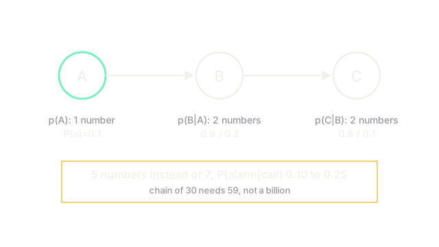
Three binary variables in a chain $A \to B \to C$ : alarm, guard checks, guard calls. Full joint: $2^3 - 1 = 7$ free numbers. Factored: $p(A)$ needs 1, $p(B \mid A)$ needs 2 (one per value of $A$ ), $p(C \mid B)$ needs 2, for $1 + 2 + 2 = 5$ numbers versus 7. Modest here; at chain length 30 it is $1 + 2 \times 29 = 59$ versus a billion.

Set $p(A{=}1) = 0.1$ , $p(B{=}1 \mid A{=}1) = 0.9$ , $p(B{=}1 \mid A{=}0) = 0.2$ , $p(C{=}1 \mid B{=}1) = 0.8$ , $p(C{=}1 \mid B{=}0) = 0.1$ . Then $p(C{=}1) = 0.8 \times p(B{=}1) + 0.1 \times p(B{=}0)$ with $p(B{=}1) = 0.9(0.1) + 0.2(0.9) = 0.27$ : $p(C{=}1) = 0.8(0.27) + 0.1(0.73) = 0.216 + 0.073 = 0.289$ . And given the call ( $C{=}1$ ), the alarm probability updates to $p(A{=}1 \mid C{=}1) = p(C{=}1 \mid A{=}1)p(A{=}1)/0.289$ where $p(C{=}1 \mid A{=}1) = 0.8(0.9) + 0.1(0.1) = 0.73$ : $0.73 \times 0.1 / 0.289 \approx 0.253$ . The call more than doubles the alarm suspicion, from 0.1 to 0.25, computed with three small tables and no joint.

Code

Elimination on the chain: two small sums replace the joint, exactly as the numbers above.

1import numpy as np2
3pA = np.array([0.9, 0.1])  # P(A=0), P(A=1)4pB_given_A = np.array([[0.8, 0.2], [0.1, 0.9]])  # rows: A value5pC_given_B = np.array([[0.9, 0.1], [0.2, 0.8]])  # rows: B value6pB = pA @ pB_given_A  # eliminate A7pC = pB @ pC_given_B  # eliminate B8print(np.round(pB, 3))  # -> [0.73 0.27]9print(round(float(pC[1]), 3))  # -> 0.289

Each @ is one variable eliminated by summing it out locally. On a 30-chain this loop replaces a billion-entry table; on a tree it is exact, and on loopy graphs it becomes loopy belief propagation, which is approximate.

Watch Out For

Cycles in a directed model

A directed cycle $A \to B \to A$ has no valid factorization: the product of conditionals is unnormalized or contradictory, and every sampler built on it produces confident nonsense. Direction must be acyclic, always. When the domain genuinely feeds back, switch to an undirected model or unroll time explicitly.

Treating the undirected normalizer as 1

Markov random field factors $\psi_c$ are not probabilities and their product does not sum to 1. Forgetting $Z$ corrupts every probability the model quotes, while leaving the argmax intact, which is why the bug survives testing on predictions and detonates on calibration. Learn with contrastive or likelihood methods that account for $Z$ .

The Quick Version

Graphical models factor a joint along a graph: one small table per node or clique.
A 3-chain needs 5 numbers instead of 7; a 30-chain needs 59 instead of a billion.
Directed models multiply conditionals on a DAG; undirected models multiply clique potentials over $Z$ .
Independence read from the graph is what makes inference algorithms fast.
The worked chain lifts alarm suspicion from 0.10 to 0.25 on observing the call.
Cycles break directed models; forgotten normalizers break undirected probabilities.