Calculus and Optimization

Calculus provides the mathematical language of instantaneous change, while optimization uses those rates to systematically steer parameters toward the lowest possible error.

Taylor series quadratic model guides parameter updates through loss landscapes toward minima.

Why Does This Exist?

Machine learning models do not learn through magical intuition; they solve numerical optimization problems. A neural network with $d$ weights is a parameterized function $f_{\mathbf{\theta}}$ , and training seeks a weight vector $\mathbf{\theta}^* \in \mathbb{R}^d$ that minimizes an empirical loss function $\mathcal{L}(\mathbf{\theta})$ .

In modern models, parameter dimension $d$ ranges from thousands to hundreds of billions. Evaluating the loss at every possible point in parameter space is physically impossible — an exhaustive grid search over just 50 parameters with 10 values each requires $10^{50}$ function evaluations. Random guessing is equally hopeless in high-dimensional space.

Calculus makes high-dimensional optimization tractable by replacing global search with local sensitivity analysis. Instead of wondering what the loss function looks like across the entire universe of weights, calculus asks a local question: if we alter each parameter by an infinitesimal amount, in what direction does the loss decline fastest, and how does the slope curve? Calculus computes the gradient and curvature, and optimization builds the iterative algorithms that ride those sensitivities to the lowest error.

For the foundations of directional derivatives and slope vectors, see our guides on derivatives and partial derivatives and gradients.

Think of It Like This

A blindfolded skier feeling slope and curvature through ski poles

Imagine standing on a snow-covered mountain in thick fog. You cannot see the valley floor, the surrounding peaks, or the distant ski lodge. Your goal is to descend to the lowest point on the mountain as quickly and safely as possible.

Your ski boots feel the tilt of the snow directly underneath you. That tilt is the first derivative — the gradient. It tells you which compass direction points downhill and how steep the immediate decline is. If you only use your boots, you take small steps in the steepest downhill direction.

Now you extend two ski poles and tap the snow five feet in front of you, behind you, and to your sides. By sensing how the slope changes between your boots and the pole tips, you detect curvature — the second derivative, represented by the Hessian. The poles tell you whether the slope is flattening out into a safe bowl, plummeting over a vertical cliff, or twisting into a treacherous mountain pass (a saddle point).

Optimization is your downhill strategy: calculus gathers the slope and curvature readings, and optimization decides how long your stride should be, when to accelerate, and when to brake to avoid crashing.

The analogy stops because mountains exist in 3 physical dimensions where gravity pulls downward automatically, whereas neural networks operate in billions of mathematical dimensions where optimization must compute its own synthetic gravity at every step.

How It Actually Works

Multivariable Taylor Approximations and Critical Points

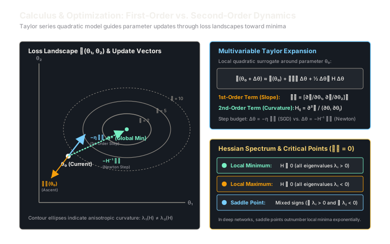
At the heart of optimization is the multivariable Taylor series expansion. For any twice-differentiable loss function $\mathcal{L}: \mathbb{R}^d \to \mathbb{R}$ , we can approximate the loss in a local neighborhood around parameter vector $\mathbf{\theta}_0$ by perturbing it with a small displacement vector $\Delta \mathbf{\theta}$ :

\mathcal{L}(\mathbf{\theta}_0 + \Delta \mathbf{\theta}) \approx \mathcal{L}(\mathbf{\theta}_0) + \nabla \mathcal{L}(\mathbf{\theta}_0)^T \Delta \mathbf{\theta} + \frac{1}{2} \Delta \mathbf{\theta}^T \mathbf{H}(\mathbf{\theta}_0) \Delta \mathbf{\theta}

where $\nabla \mathcal{L}(\mathbf{\theta}_0) \in \mathbb{R}^d$ is the gradient vector of first-order partial derivatives:

\nabla \mathcal{L}(\mathbf{\theta}_0) = \left[ \frac{\partial \mathcal{L}}{\partial \theta_1}, \frac{\partial \mathcal{L}}{\partial \theta_2}, \dots, \frac{\partial \mathcal{L}}{\partial \theta_d} \right]^T

and $\mathbf{H}(\mathbf{\theta}_0) \in \mathbb{R}^{d \times d}$ is the symmetric Hessian matrix of second-order partial derivatives:

H_{ij} = \frac{\partial^2 \mathcal{L}}{\partial \theta_i \partial \theta_j}

The gradient provides the tangent hyperplane (local linear trend), while the Hessian provides the osculating paraboloid (local curvature).

First-Order Optimization: Gradient Descent

If we truncate the Taylor expansion to first order and add an $L_2$ step-size penalty $\frac{1}{2\eta} \|\Delta \mathbf{\theta}\|^2$ to keep the displacement within the valid local trust region, we minimize:

\min_{\Delta \mathbf{\theta}} \left( \nabla \mathcal{L}(\mathbf{\theta}_0)^T \Delta \mathbf{\theta} + \frac{1}{2\eta} \|\Delta \mathbf{\theta}\|^2 \right)

Differentiating with respect to $\Delta \mathbf{\theta}$ and setting to zero yields the foundational Gradient Descent update rule:

\Delta \mathbf{\theta} = -\eta \nabla \mathcal{L}(\mathbf{\theta}_0) \implies \mathbf{\theta}_{t+1} = \mathbf{\theta}_t - \eta \nabla \mathcal{L}(\mathbf{\theta}_t)

where $\eta > 0$ is the learning rate.

Second-Order Optimization: Newton's Method

If we include the quadratic term and differentiate the full second-order Taylor approximation with respect to $\Delta \mathbf{\theta}$ :

\nabla_{\Delta \mathbf{\theta}} \left( \mathcal{L}(\mathbf{\theta}_0) + \nabla \mathcal{L}(\mathbf{\theta}_0)^T \Delta \mathbf{\theta} + \frac{1}{2} \Delta \mathbf{\theta}^T \mathbf{H} \Delta \mathbf{\theta} \right) = \nabla \mathcal{L}(\mathbf{\theta}_0) + \mathbf{H} \Delta \mathbf{\theta} = \mathbf{0}

Solving for $\Delta \mathbf{\theta}$ gives the Newton-Raphson update:

\Delta \mathbf{\theta} = -\mathbf{H}(\mathbf{\theta}_0)^{-1} \nabla \mathcal{L}(\mathbf{\theta}_0) \implies \mathbf{\theta}_{t+1} = \mathbf{\theta}_t - \mathbf{H}(\mathbf{\theta}_t)^{-1} \nabla \mathcal{L}(\mathbf{\theta}_t)

Newton's method rescales the step by the inverse curvature along every eigen-axis, jumping directly to the minimum of a quadratic bowl in a single step without needing a manual learning rate.

Critical Point Classification

A point where the gradient vanishes ( $\nabla \mathcal{L}(\mathbf{\theta}^*) = \mathbf{0}$ ) is a stationary (critical) point. The eigenvalues $\lambda_1, \lambda_2, \dots, \lambda_d$ of the Hessian matrix $\mathbf{H}(\mathbf{\theta}^*)$ determine its geometric identity:

Local Minimum: $\mathbf{H} \succ 0$ (all $\lambda_i > 0$ , positive definite). The surface curves upward in every direction.
Local Maximum: $\mathbf{H} \prec 0$ (all $\lambda_i < 0$ , negative definite). The surface curves downward in every direction.
Saddle Point: $\mathbf{H}$ is indefinite (at least one $\lambda_i > 0$ and at least one $\lambda_j < 0$ ). The surface rises along some axes and falls along others.

Worked Example

Consider minimizing the anisotropic quadratic loss function:

\mathcal{L}(\theta_1, \theta_2) = 2\theta_1^2 + \theta_2^2 - 4\theta_1 - 2\theta_2 + 5

Starting at the origin $\mathbf{\theta}_0 = [0, 0]^T$ :

Compute first-order partial derivatives:
$\frac{\partial \mathcal{L}}{\partial \theta_1} = 4\theta_1 - 4, \quad \frac{\partial \mathcal{L}}{\partial \theta_2} = 2\theta_2 - 2$
At $\mathbf{\theta}_0 = [0, 0]^T$ , the gradient is:
$\nabla \mathcal{L}(0, 0) = \begin{bmatrix} 4(0) - 4 \\ 2(0) - 2 \end{bmatrix} = \begin{bmatrix} -4 \\ -2 \end{bmatrix}$
Compute the second-order Hessian matrix:
$\mathbf{H} = \begin{bmatrix} \frac{\partial^2 \mathcal{L}}{\partial \theta_1^2} & \frac{\partial^2 \mathcal{L}}{\partial \theta_1 \partial \theta_2} \\ \frac{\partial^2 \mathcal{L}}{\partial \theta_2 \partial \theta_1} & \frac{\partial^2 \mathcal{L}}{\partial \theta_2^2} \end{bmatrix} = \begin{bmatrix} 4 & 0 \\ 0 & 2 \end{bmatrix}$
The eigenvalues are $\lambda_1 = 4$ and $\lambda_2 = 2$ . Both are positive, proving $\mathbf{H} \succ 0$ everywhere (strictly convex).
First-order step with learning rate $\eta = 0.1$ :
$\mathbf{\theta}_1 = \mathbf{\theta}_0 - \eta \nabla \mathcal{L}(\mathbf{\theta}_0) = \begin{bmatrix} 0 \\ 0 \end{bmatrix} - 0.1 \begin{bmatrix} -4 \\ -2 \end{bmatrix} = \begin{bmatrix} 0.4 \\ 0.2 \end{bmatrix}$
Initial loss: $\mathcal{L}(0, 0) = 5.0$ . New loss:
$\mathcal{L}(0.4, 0.2) = 2(0.4)^2 + (0.2)^2 - 4(0.4) - 2(0.2) + 5 = 0.32 + 0.04 - 1.6 - 0.4 + 5 = 3.36$
The loss drops from $5.0$ to $3.36$ .
Second-order Newton step: The inverse Hessian is:
$\mathbf{H}^{-1} = \begin{bmatrix} 4 & 0 \\ 0 & 2 \end{bmatrix}^{-1} = \begin{bmatrix} 0.25 & 0 \\ 0 & 0.5 \end{bmatrix}$
The exact Newton displacement is:
$\Delta \mathbf{\theta}_{\text{Newton}} = -\mathbf{H}^{-1} \nabla \mathcal{L}(\mathbf{\theta}_0) = -\begin{bmatrix} 0.25 & 0 \\ 0 & 0.5 \end{bmatrix} \begin{bmatrix} -4 \\ -2 \end{bmatrix} = \begin{bmatrix} 1.0 \\ 1.0 \end{bmatrix}$
New parameter: $\mathbf{\theta}_{\text{Newton}} = [0, 0]^T + [1.0, 1.0]^T = [1.0, 1.0]^T$ . Evaluating the gradient at this new point:
$\nabla \mathcal{L}(1.0, 1.0) = \begin{bmatrix} 4(1.0) - 4 \\ 2(1.0) - 2 \end{bmatrix} = \begin{bmatrix} 0 \\ 0 \end{bmatrix}$
Newton's method reaches the exact global minimum in a single step with optimal loss $\mathcal{L}(1, 1) = 2(1) + 1 - 4 - 2 + 5 = 2.0$ .

Code

1import numpy as np2
3
4def loss_and_grad(theta: np.ndarray) -> tuple[float, np.ndarray]:5    """Compute quadratic loss and analytic gradient for theta = [theta_1, theta_2]."""6    t1, t2 = theta[0], theta[1]7    loss = float(2 * t1**2 + t2**2 - 4 * t1 - 2 * t2 + 5)8    grad = np.array([4 * t1 - 4, 2 * t2 - 2], dtype=float)9    return loss, grad10
11
12# Constant Hessian for quadratic loss13hessian = np.array([[4.0, 0.0], [0.0, 2.0]])14inv_hessian = np.linalg.inv(hessian)15
16theta_0 = np.array([0.0, 0.0])17l0, g0 = loss_and_grad(theta_0)18print(f"Initial loss: {l0:.2f}, grad: {g0}")19# -> Initial loss: 5.00, grad: [-4. -2.]20
21# 1. Gradient Descent Step (lr = 0.1)22lr = 0.123theta_gd = theta_0 - lr * g024l_gd, g_gd = loss_and_grad(theta_gd)25print(f"GD step: theta = {theta_gd}, loss = {l_gd:.2f}")26# -> GD step: theta = [0.4 0.2], loss = 3.3627
28# 2. Newton's Method Step29theta_newton = theta_0 - inv_hessian @ g030l_newton, g_newton = loss_and_grad(theta_newton)31print(f"Newton step: theta = {theta_newton}, loss = {l_newton:.2f}")32# -> Newton step: theta = [1. 1.], loss = 2.0033print(f"Newton residual gradient: {g_newton}")34# -> Newton residual gradient: [0. 0.]

Watch Out For

Second-order Newton steps leaping toward saddle points and maxima

Newton's method seeks stationary points where $\nabla \mathcal{L} = \mathbf{0}$ , but it is completely blind to whether that stationary point is a minimum or maximum. The update $\Delta \mathbf{\theta} = -\mathbf{H}^{-1} \nabla \mathcal{L}$ inverts the Hessian unconditionally.

If the local Hessian possesses negative eigenvalues ( $\lambda_i < 0$ ), the local curvature is convex downward. In those directions, Newton's update flips sign and steps directly toward the local maximum or saddle ridge, accelerating away from lower loss regions. Furthermore, computing and inverting an exact $d \times d$ Hessian matrix requires $O(d^3)$ arithmetic, which is intractable when $d > 10^5$ .

Fix: In high-dimensional non-convex optimization, prefer first-order methods with momentum (such as Adam), or use quasi-Newton trust-region methods (like L-BFGS with damping) that maintain positive-definite Hessian approximations and enforce descent conditions before taking a step.

The Quick Version

Calculus provides the gradient $\nabla \mathcal{L}$ for local slope direction and the Hessian $\mathbf{H}$ for multivariable curvature.
Gradient descent follows the negative gradient direction with step size $\eta$ , trading second-order speed for linear $O(d)$ computational efficiency per step.
Newton's method uses the inverse Hessian $\mathbf{H}^{-1}$ to eliminate curvature scale imbalances, reaching the minimum of a quadratic function in one step.
Stationary points where $\nabla \mathcal{L} = \mathbf{0}$ are classified by Hessian eigenvalues: all positive indicates a minimum, all negative a maximum, and mixed signs a saddle point.
Modern deep learning relies predominantly on first-order stochastic methods because inverting large Hessians is computationally prohibitive and prone to saddle-point attraction.