Convex and Non-Convex Optimization

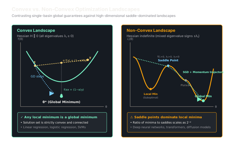
In convex optimization any local minimum is guaranteed to be global, while non-convex optimization navigates rugged landscapes packed with saddle points and spurious valleys.

Contrasting a convex bowl with a single global optimum against a rugged non-convex loss landscape containing local minima, saddle points, and plateaus.

Why Does This Exist?

The great watershed in optimization theory is not between linearity and non-linearity, but between convexity and non-convexity.

In classical machine learning — ordinary least squares, logistic regression, and Support Vector Machines — models are deliberately formulated as convex optimization problems. For a convex function, any local minimum is mathematically guaranteed to be a global minimum. Solvers initialized from arbitrary starting points converge reliably to the exact optimal parameters without babysitting or stochastic tricks.

Modern deep neural networks shatter this guarantee. The composition of multiple non-linear activation layers, batch normalization, attention mechanisms, and weight permutation symmetries turns the loss surface into an intensely non-convex landscape. It contains billions of parameters, flat plateaus, local minima, and an astronomical number of saddle points where slopes vanish in all directions but curve downwards along certain escape corridors.

Understanding the boundary between convex and non-convex optimization explains why deep learning practitioners cannot rely on traditional second-order solvers, why careful weight initialization is mandatory, and how stochastic noise enables gradient descent to escape deceptive saddle points.

For the mathematical definitions of convex domains, explore our guide on convex sets and functions.

Think of It Like This

A smooth salad bowl vs. an expansive mountain range

Imagine dropping a steel marble into a smooth ceramic salad bowl. No matter where you release it on the rim, gravity guides the marble directly to the single lowest point at the bottom center. There are no secondary traps, no false basins, and no deceptive flat ledges. That is convex optimization: simple downhill momentum is guaranteed to discover the absolute global best outcome.

Now imagine dropping that same marble into a rugged mountain range covered in dense fog. The marble can settle into an elevated mountain lake thousands of feet above the actual valley floor (a suboptimal local minimum). It can roll onto an enormous flat mesa where gravity barely exerts any pull (a vanishing gradient plateau). Or it can pause on a mountain pass — a saddle ridge that slopes uphill to your left and right, but drops downhill in front and behind you.

In the mountains, simple passive rolling is not enough. You need explosive tremors to bounce out of shallow traps, and directional momentum to ride through narrow mountain passes down to the deep valley below. That is non-convex optimization.

The analogy stops because mountains exist in 3 physical dimensions where local minima traps are common. In neural networks with millions of dimensions, true trapped local minima are surprisingly rare; saddle points outnumber local minima exponentially.

How It Actually Works

Convexity Conditions and High-Dimensional Saddle Proliferation

Mathematically, a function $f: \mathbb{R}^d \to \mathbb{R}$ is defined as convex if its domain is a convex set and for all points $\mathbf{x}, \mathbf{y} \in \text{dom}(f)$ and any scalar $\alpha \in [0, 1]$ :

f(\alpha \mathbf{x} + (1-\alpha)\mathbf{y}) \le \alpha f(\mathbf{x}) + (1-\alpha) f(\mathbf{y})

Geometrically, the straight line chord connecting $( \mathbf{x}, f(\mathbf{x}) )$ and $( \mathbf{y}, f(\mathbf{y}) )$ always sits on or above the graph of $f$ .

For twice continuously differentiable functions, convexity is characterized by the curvature of the second derivative. Function $f$ is convex if and only if its Hessian matrix $\nabla^2 f(\mathbf{x})$ is positive semi-definite everywhere:

\nabla^2 f(\mathbf{x}) \succeq 0 \quad \forall \mathbf{x} \iff \lambda_{\min}(\nabla^2 f(\mathbf{x})) \ge 0

where $\lambda_{\min}$ is the smallest eigenvalue of the Hessian. If $\nabla^2 f(\mathbf{x}) \succ 0$ (strictly positive definite), the function is strictly convex and its global minimizer is strictly unique.

The Non-Convex Landscape and Critical Points

In non-convex functions, the Hessian matrix is indefinite: its eigenvalues take both positive and negative values depending on position. At any critical point where the gradient vanishes ( $\nabla f(\mathbf{x}) = \mathbf{0}$ ):

Local Minimum: All eigenvalues are strictly positive ( $\lambda_i > 0$ for all $i = 1, \dots, d$ ).
Local Maximum: All eigenvalues are strictly negative ( $\lambda_i < 0$ for all $i = 1, \dots, d$ ).
Saddle Point: The Hessian has at least one positive eigenvalue and at least one negative eigenvalue ( $\exists \lambda_i > 0, \exists \lambda_j < 0$ ).

Why Saddles Dominate Deep Learning

In a $d$ -dimensional space, consider a random critical point where the eigenvalues of the Hessian are distributed around zero with roughly equal chance of being positive or negative. The probability that all $d$ eigenvalues happen to be simultaneously positive (forming a true local minimum) is:

P(\text{local minimum}) \approx \left(\frac{1}{2}\right)^d = 2^{-d}

For a small network with $d = 10,000$ parameters, $2^{-10000} \approx 0$ . True local minima are virtually non-existent at high loss values! Instead, critical points at elevated loss values are overwhelmingly saddle points. First-order methods equipped with stochastic noise or momentum can follow the negative eigenvalue directions ( $\lambda_j < 0$ ) to escape these saddles and descend toward flat, wide basins where loss is low.

Worked Example

Let us examine two concrete functions at their critical points:

1. Convex Quadratic Function

Consider $f_1(x_1, x_2) = 2x_1^2 + x_2^2 + 4x_1 - 6x_2 + 15$ . First, find the gradient:

\nabla f_1 = \begin{bmatrix} 4x_1 + 4 \\ 2x_2 - 6 \end{bmatrix}

Setting $\nabla f_1 = \mathbf{0}$ yields $4x_1 + 4 = 0 \implies x_1^* = -1$ and $2x_2 - 6 = 0 \implies x_2^* = 3$ . The critical point is $\mathbf{x}^* = [-1, 3]^T$ . Compute the Hessian:

\mathbf{H}_1 = \begin{bmatrix} 4 & 0 \\ 0 & 2 \end{bmatrix}

The eigenvalues are $\lambda_1 = 4 > 0$ and $\lambda_2 = 2 > 0$ . Because $\mathbf{H}_1 \succ 0$ everywhere, $f_1$ is strictly convex across all of $\mathbb{R}^2$ , and $\mathbf{x}^* = [-1, 3]^T$ is the unique global minimum with optimal value:

f_1(-1, 3) = 2(-1)^2 + (3)^2 + 4(-1) - 6(3) + 15 = 2 + 9 - 4 - 18 + 15 = 4

2. Non-Convex Saddle Function

Consider the hyperbolic paraboloid (saddle surface):

f_2(x_1, x_2) = x_1^2 - 3x_2^2

Compute the gradient:

\nabla f_2 = \begin{bmatrix} 2x_1 \\ -6x_2 \end{bmatrix}

Setting $\nabla f_2 = \mathbf{0}$ yields the critical point at the origin $(0, 0)$ . Compute the Hessian:

\mathbf{H}_2 = \begin{bmatrix} 2 & 0 \\ 0 & -6 \end{bmatrix}

The eigenvalues are $\lambda_1 = +2$ and $\lambda_2 = -6$ . Along the $x_1$ -axis ( $x_2 = 0$ ), $f_2(x_1, 0) = x_1^2$ , which curves upward with minimum at $0$ . Along the $x_2$ -axis ( $x_1 = 0$ ), $f_2(0, x_2) = -3x_2^2$ , which curves downward with maximum at $0$ . Because eigenvalues have opposite signs, $(0, 0)$ is a strict saddle point. Any perturbation along $x_2$ triggers catastrophic descent toward $-\infty$ .

Code

1import numpy as np2
3
4def analyze_critical_point(5    hessian: np.ndarray,6) -> tuple[str, np.ndarray, bool]:7    """Classify a critical point using Hessian eigenvalues and test convexity."""8    eigenvalues = np.linalg.eigvalsh(hessian)9
10    all_positive = bool(np.all(eigenvalues > 1e-8))11    all_negative = bool(np.all(eigenvalues < -1e-8))12    has_mixed = bool(np.any(eigenvalues > 1e-8) and np.any(eigenvalues < -1e-8))13
14    if all_positive:15        point_type = "Local/Global Minimum"16        is_convex = True17    elif all_negative:18        point_type = "Local Maximum"19        is_convex = False20    elif has_mixed:21        point_type = "Saddle Point"22        is_convex = False23    else:24        point_type = "Degenerate / Valley"25        is_convex = bool(np.all(eigenvalues >= -1e-8))26
27    return point_type, eigenvalues, is_convex28
29
30# 1. Strictly Convex System31h_convex = np.array([[4.0, 0.0], [0.0, 2.0]])32pt_type_1, eigs_1, is_cvx_1 = analyze_critical_point(h_convex)33print(f"H1 -> {pt_type_1}, eigs={eigs_1}, convex={is_cvx_1}")34# -> H1 -> Local/Global Minimum, eigs=[2. 4.], convex=True35
36# 2. Non-Convex Saddle System37h_saddle = np.array([[2.0, 0.0], [0.0, -6.0]])38pt_type_2, eigs_2, is_cvx_2 = analyze_critical_point(h_saddle)39print(f"H2 -> {pt_type_2}, eigs={eigs_2}, convex={is_cvx_2}")40# -> H2 -> Saddle Point, eigs=[-6.  2.], convex=False41
42# Simulated escape step along negative curvature eigenvector43neg_idx = int(np.argmin(eigs_2))44eigvec_escape = np.array([0.0, 1.0])  # Eigenvector for lambda = -645step = 0.1 * eigvec_escape46f_before = 0.0  # at origin47f_after = float(step[0] ** 2 - 3 * step[1] ** 2)48print(f"Escaping saddle: f drops from {f_before:.2f} to {f_after:.4f}")49# -> Escaping saddle: f drops from 0.00 to -0.0300

Watch Out For

Mistaking high-dimensional saddle plateaus for bad local minima

When training loss plateaus, machine learning practitioners often conclude that their neural network is trapped in a bad local minimum. In practice, genuine bad local minima (critical points where all eigenvalues are strictly positive with high loss) are extraordinarily rare in over-parameterized neural networks.

What actually stalls training is a high-dimensional saddle point or an ill-conditioned ravine where the gradient norm $\|\nabla \mathcal{L}\|$ drops below $10^{-5}$ along flat directions. Vanilla gradient descent crawls painfully slowly along the flat ridge because the gradient provides virtually no driving force.

Fix: Do not increase model capacity to bypass presumed local minima. Instead, introduce momentum (such as Polyak momentum or Adam), reduce the mini-batch size to increase stochastic gradient noise (which naturally perturbs weights along negative curvature escape directions), or use learning rate warm-up and cosine annealing schedules.

The Quick Version

Convex optimization ensures that any stationary point with zero gradient is a global minimum, verified by a positive semi-definite Hessian $\nabla^2 f \succeq 0$ .
Deep neural networks possess non-convex loss surfaces where multiple weight configurations yield identical outputs due to permutation symmetries.
In high dimensions ( $d \gg 1$ ), critical points with elevated loss are exponentially dominated by saddle points rather than local minima ( $2^{-d}$ probability).
Escaping non-convex saddles relies on stochastic mini-batch perturbations and momentum, which follow negative curvature directions downhill.
Convex formulations remain the bedrock of statistical machine learning, providing exact convergence rates and global certificates where deep models offer only empirical convergence.