Convex Sets and Convex Functions

A convex set keeps every segment between its points inside itself, and a convex function sits below all its chords, which together guarantee a single global bottom.

A disk keeps the segment between two of its points inside with midpoint norm 0.707, and the chord between x equals 1 and 3 on x squared sits at 5 above the curve value 4

Why Does This Exist?

Optimisation needs a promise: that the search cannot get stuck somewhere that merely looks best nearby. Convex sets and convex functions are that promise, split into two halves. The set half says the ground you search over has no holes or dents that trap you. The function half says the surface you descend has exactly one bottom.

Without the pair, every algorithm needs restarts, luck, or exhaustive search. With it, linear regression, logistic regression, SVMs and lasso all converge to the same answer from any start, and a single local check certifies the global optimum. This page defines both halves and proves the guarantee; convex optimization then builds the algorithms and certificates on top, and convexity and loss landscapes shows what breaks when networks leave this world.

The one idea you need first

A line segment between points $a$ and $b$ is the set of weighted averages $ta + (1-t)b$ for $t \in [0, 1]$ . At $t = 0.5$ you get the midpoint. Everything on this page is a statement about where those averages land.

Think of It Like This

A walled lake versus two separate ponds

A convex set is a walled lake: stand anywhere in the water with a friend anywhere else, stretch a rope between you, and the whole rope stays wet. The midpoint of any two swimmers is still swimming.

Now drain the middle so only two separate ponds remain. Two swimmers in different ponds stretch their rope across dry grass: the midpoint left the set. That pair of ponds is non-convex, and an optimiser wading downhill can be stranded in the wrong pond with no path to the better one.

A convex function adds the matching surface rule: the lakebed between any two soundings never bulges above the straight line joining them. No hidden ridge can dam the descent.

Where the analogy stops: real lakes are two-dimensional, where you can see the dent. In high dimensions the dent is invisible and the test is algebraic, the segment formula and the chord inequality, not eyesight.

How It Actually Works

Convex sets

A set $C$ is convex when the segment between any two of its points stays inside it:

a, b \in C \implies ta + (1-t)b \in C \quad \forall t \in [0, 1]

Examples: the unit disk, any line or hyperplane, the set of matrices with bounded norm. Non-examples: two separate disks, a crescent, any set with a hole. Intersections of convex sets stay convex, which is why adding convex constraints keeps a problem convex.

Convex functions

A function $f$ on a convex domain is convex when its graph sits below every chord:

f(ta + (1-t)b) \le tf(a) + (1-t)f(b) \quad \forall t \in [0, 1]

The special case $t = 0.5$ is Jensen's inequality for two points: $f$ of the average never exceeds the average of $f$ . For twice-differentiable $f$ the working test is curvature: convex exactly when the Hessian is positive semi-definite everywhere, the same positive-definite machinery the landscape pages use.

Why one bottom follows

Suppose $x^\star$ is a local minimum but some $y$ is better: $f(y) < f(x^\star)$ . Walk the segment from $x^\star$ toward $y$ . Convexity forces $f$ along the segment below the chord, so arbitrarily close to $x^\star$ there are points with value below $f(x^\star)$ , contradicting local minimality. Hence every local minimum is global. The gradient being zero, or KKT holding under constraints, then certifies the answer instead of merely suggesting it.

Worked example

Both halves, with numbers small enough to check by hand.

Set. Take the unit disk $C = \{(x_1, x_2) : x_1^2 + x_2^2 \le 1\}$ with $a = (1, 0)$ and $b = (0, 1)$ , both on the boundary since $1^2 + 0^2 = 1$ . The midpoint is $m = (0.5, 0.5)$ with squared norm $0.5^2 + 0.5^2 = 0.25 + 0.25 = 0.5 \le 1$ , so $m \in C$ with norm $\sqrt{0.5} \approx 0.707$ . The segment stayed inside, as the diagram shows. Contrast the two-point set $S = \{(1, 0), (0, 1)\}$ : the same midpoint $(0.5, 0.5)$ is not in $S$ at all, so $S$ is not convex.

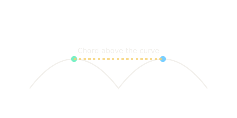
Function. Take $f(x) = x^2$ with $a = 1$ , $b = 3$ , $t = 0.5$ . The midpoint is $m = 2$ with $f(m) = 4$ . The chord average is $(f(1) + f(3))/2 = (1 + 9)/2 = 5$ . Since $4 \le 5$ , the chord sits above the curve, confirming convexity at this pair with a gap of exactly 1.

Code

1import numpy as np2
3
4def in_unit_disk(p: np.ndarray) -> bool:5    return float(p @ p) <= 1.0 + 1e-126
7
8a = np.array([1.0, 0.0])9b = np.array([0.0, 1.0])10m = 0.5 * a + 0.5 * b11print(m, round(float(m @ m), 4), in_unit_disk(m))12# -> [0.5 0.5] 0.5 True   midpoint norm^2 is 0.5, inside the disk13
14def f(x: float) -> float:15    return x ** 216
17
18mid, chord = f(0.5 * (1 + 3)), (f(1) + f(3)) / 219print(mid, chord, mid <= chord)20# -> 4.0 5.0 True   curve below chord, gap of 1.0

The disk check prints norm-squared $0.5$ and True; the chord check prints $4.0$ against $5.0$ , the same gap the diagram draws.

Watch Out For

Assuming a convex function over any domain is a convex problem

Convexity of the function alone is not enough: the domain must be convex too. Minimising $x^2$ over the two-point set $\{(1, 0), (0, 1)\}$ from the worked example has no segment to descend along, and "local versus global" stops meaning anything. Optimisers assume they can step toward a better point and stay feasible; a non-convex domain breaks that step.

Always check both halves before claiming the guarantee: convex objective and convex feasible set. If the domain is discrete, disconnected, or holed, you have a combinatorial or non-convex problem wearing convex clothes.

Reading Jensen backwards on concave objectives

For concave functions such as the logarithm, the inequality flips: $f$ of the average exceeds the average of $f$ . Applying the convex direction to a concave utility or log-likelihood silently reverses a bound, turning a valid lower bound into an invalid one and an EM or variational argument into nonsense.

Check the curvature sign first. If $f'' < 0$ , you hold a concave function and the chord sits below the graph. Misreading the direction is the most common way a correct-looking derivation produces an impossible number, such as a "lower bound" above the true value.

The Quick Version

A set is convex when every segment between its points stays inside it; intersections preserve this.
A function is convex when its graph sits below every chord, equivalently a positive semi-definite Hessian.
Jensen at two points: $f$ of the average never exceeds the average of $f$ .
Every local minimum of a convex function over a convex set is global.
Unit disk midpoint $(0.5, 0.5)$ has norm about $0.707$ and stays inside; the same pair as a bare two-point set fails.
On $x^2$ between 1 and 3, the curve gives 4 against a chord of 5, a gap of 1.
Convex function plus non-convex domain is not a convex problem; check both halves.
Concave functions flip Jensen, so confirm the curvature sign before bounding.