Girsanov Theorem

Changing drift is changing measure: tilt Brownian paths by an exponential weight and a new drift appears. Likelihood ratios between diffusions come from that weight.

Tilting flat Brownian paths by an exponential weight shifts their mean by 1.0 over 2 units at a KL cost of 0.25 nats

Why Does This Exist?

Diffusion models, likelihood evaluation and importance sampling all compare two path measures: noise versus data-driven drift, proposal versus target sampler, prior versus posterior diffusion. Simulating both and ratioing histograms is hopeless in path space. What you need is the exact likelihood ratio between two diffusions sharing volatility but differing in drift.

Girsanov supplies it. Under a new measure defined by an exponential martingale weight, a Brownian motion gains a drift, or equivalently a drifted process becomes Brownian. The KL between the measures is half the integrated squared drift difference. That formula prices guided generation, evidence bounds and sampler comparisons in nats.

Prerequisite in one paragraph. You need absolute continuity (two measures agreeing on impossible events) and the exponential martingale $Z = \exp(\int \theta\,dW - \frac{1}{2}\int \theta^2\,dt)$ with market price of risk $\theta$ . Background is in Brownian motion and probability distributions.

Think of It Like This

Handicapping a fair coin after the tosses

Toss a fair coin $100$ times and record heads. To pretend the coin favoured heads at $60$ percent, reweight each sequence by $(1.2)^{\text{heads}}(0.8)^{\text{tails}}$ : sequences with many heads gain weight, others lose it. Under the tilted weights the coin looks biased, though no toss changed.

Girsanov reweights paths the same way continuously. The weight tilts flat Brownian wiggles into drifted ones. The KL cost is the log-average weight, measuring how far the pretence stretches.

Where the analogy stops: coin weights are bounded products while Girsanov weights are stochastic exponentials needing Novikov integrability. Unweighted tails can also break the martingale into a strict local martingale, voiding the change.

How It Actually Works

Let $W$ be Brownian under $P$ and $\theta_t$ adapted with $E[\exp(\frac{1}{2}\int_0^T \theta_t^2\,dt)] < \infty$ (Novikov). Define $dQ/dP = \exp(\int_0^T \theta_t\,dW_t - \frac{1}{2}\int_0^T \theta_t^2\,dt)$ . Then $\tilde{W}_t = W_t - \int_0^t \theta_s\,ds$ is Brownian under $Q$ : paths gain drift $\theta$ under the tilt. Flipped, an SDE $dX = \mu\,dt + dW$ under $P$ becomes $dX = (\mu + \theta)\,dt + d\tilde{W}$ under $Q$ .

For constant drifts $0$ versus $a$ over $T$ , $KL(Q\|P) = a^2T/2$ .

Worked example

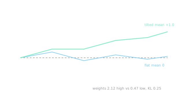
Add drift $a = 0.5$ over $T = 2$ to unit Brownian. Then $KL = 0.25 \times 2/2 = 0.25$ nats. The weight is $\exp(0.5W_2 - 0.25)$ : a path ending at $W_2 = 2.0$ gets weight $\exp(1.0 - 0.25) = \exp(0.75) \approx 2.12$ , while one ending at $-1.0$ gets $\exp(-0.5 - 0.25) = \exp(-0.75) \approx 0.47$ . Tilted mean moves $aT = 1.0$ right, matching the diagram. Guided diffusion pays similar nats per unit drift squared when strengthening conditioning.

Watch Out For

Tilting with a non-integrable market price

With $\theta_t = 1/(T-t)$ exploding at the horizon, the Novikov expectation diverges and $Z$ is a strict local martingale with mean below $1$ . The supposed $Q$ leaks mass and likelihood ratios do not integrate to one, silently biasing evidence estimates downward.

Fix: verify Novikov or Kazamaki before changing measure. Cap or localise explosive drifts.

Changing volatility by measure change

Girsanov changes drift only; volatility is invariant under equivalent changes. Trying to remove $0.5$ volatility by tilting leaves paths mutually singular: likelihood ratios of zero or infinity and KL infinite. Volatility differences need entirely different tools.

Fix: match volatilities before Girsanov. Drift is negotiable, diffusion is not.

The Quick Version

Girsanov tilts path measure by a stochastic exponential, turning drift into weight and back.
Constant drift $0.5$ over $2$ units costs KL $0.25$ nats and shifts means by $1.0$ .
Paths ending high gain weight $2.12$ ; paths ending low fall to $0.47$ in the example.
Novikov integrability is mandatory, otherwise the new measure leaks mass.
Drift changes measure; volatility never does under equivalence.