Joint, Marginal and Conditional Distributions

The joint table holds everything. Add across a row to ignore a variable, or zoom into one row to learn from it. Those two moves run all of inference.

A two-by-two joint table with row sums 0.6 and 0.4, and the Y equals 1 column rescaled by 0.4 into the conditional split 0.25 and 0.75

Why Does This Exist?

Data comes joint and questions come sliced. Sensors report feature-label pairs together, but deployment asks about labels given features. Trials record treatment, recovery, and age together, but policy asks about recovery given treatment. The joint distribution holds every answer at once, and marginalization plus conditioning extract the one you need.

These two moves divide the whole field. Summing a variable out ignores it, which is how intractable nuisances get removed and how Bayes' theorem denominators get computed. Conditioning zooms into what was observed, which is what every classifier outputs: probability foundations defines a classifier as exactly such a conditional. Mixture models, EM, and Gibbs sampling are all choreography of these two steps.

The one idea you need first

A joint chance $P(X = x, Y = y)$ is the fraction of outcomes where both hold. Fix $Y = y$ and re-normalize the survivors to total one: that is the conditional $P(X \mid Y = y)$ . Add the joint over all $y$ instead and $Y$ disappears: that is the marginal $P(X)$ . Slice versus sum, zoom versus ignore.

Think of It Like This

A school roster and two questions

The roster lists every student with grade and sport. Ask what fraction plays soccer and you scan the whole roster: the marginal. Ask what fraction of tenth-graders plays soccer and you first filter to tenth grade, then scan within: the conditional.

Filtering before counting is the entire difference. The roster never changes, but the question selects its audience. Forgetting to re-normalize after filtering counts tenth-grade soccer players against the whole school, understating by the filter's share. Every conditioning bug is some version of counting a filtered audience against an unfiltered crowd.

The analogy stops at observation. Rosters are complete and exact, while real joints are estimated from samples, so both the sums and the slices inherit sampling noise that a roster never has.

How It Actually Works

Three objects, two moves. The joint $P(X, Y)$ weighs every combination. The marginal removes a variable by the sum rule:

P(X = x) = \sum_y P(X = x, Y = y)

In plain words: add the row. The variable disappears because every one of its values was counted. The conditional zooms by re-normalizing a slice:

P(X = x \mid Y = y) = \frac{P(X = x, Y = y)}{P(Y = y)}

In plain words: keep only the $y$ outcomes and stretch them to total one. Continuous variables replace sums with integrals, and the expectation versions average against these sliced weights.

Two facts organize practice. First, marginals can match while joints differ wildly, so passing marginal checks never validates a joint model. Second, conditioning and marginalizing do not commute with nonlinear operations generally: the average of conditionals is the marginal, but the mode of conditionals need not be the marginal mode.

Worked example

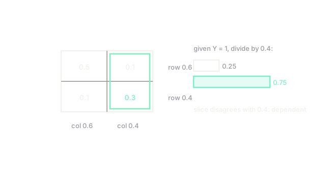
Take the joint table $P(0,0) = 0.5$ , $P(0,1) = 0.1$ , $P(1,0) = 0.1$ , $P(1,1) = 0.3$ .

Marginals by summing: $P(X = 1) = 0.1 + 0.3 = 0.4$ and $P(Y = 1) = 0.1 + 0.3 = 0.4$ . Symmetric profiles, each 0.4.

Conditionals by slicing: given $Y = 1$ , re-normalize its column total $0.4$ . Then $P(X = 1 \mid Y = 1) = 0.3 / 0.4 = 0.75$ , nearly double the marginal $0.4$ . Knowing $Y$ moved the belief sharply, which is dependence quantified: the slice disagrees with the profile. If they had agreed at $0.4$ , the variables would be independent.

Code

Marginalize and condition a joint table stored as a dictionary, the same two moves in code.

1joint = {(0, 0): 0.5, (0, 1): 0.1, (1, 0): 0.1, (1, 1): 0.3}2
3
4def marginal_y(y: int) -> float:5    return joint[(0, y)] + joint[(1, y)]  # sum the column away6
7
8def cond_x_given_y(x: int, y: int) -> float:9    return joint[(x, y)] / marginal_y(y)  # slice, then re-normalize10
11
12print(marginal_y(1))                 # -> 0.413print(round(cond_x_given_y(1, 1), 2))  # -> 0.75

The prints give 0.4 and 0.75, matching the hand computation. Note what the code never does: it never divides by anything but the slice total, which is the re-normalization beginners forget.

Watch Out For

Conditioning without re-normalizing

Slicing the joint to the observed row and reading raw joint values as answers understates every chance by the slice's share. The column summed to $0.4$ , so raw readings are all two-and-a-half times too small. Always divide by the slice total, and assert your conditionals sum to one as a standing check.

Marginalizing away the variable the question is about

Summing out the target feels productive because the table gets smaller, but the answer lives in the removed dimension. Compute the marginal of what you observe and the conditional of what you want; reversing them answers how likely the evidence is rather than how likely the hypothesis is, which is the prosecutor's fallacy in one line.

The Quick Version

The joint weighs every combination; everything else is derived from it.
Marginalization sums a variable away and ignores it; conditioning slices to observations and learns from them.
Conditionals must re-normalize by the slice total, or every answer is short by the slice's share.
In the worked table, Y equal to 1 lifts X toward 0.75 against a marginal of 0.4, which is dependence.
Matching marginals never validate a joint: different togetherness hides behind identical profiles.