Spectral Graph Theory

Reading a graph through the eigenvalues of its matrices: what the spectrum guarantees about cuts, clusters, and spreading without any search.

A triangle with Laplacian spectrum 0, 3, 3 is spectrally far better knit than a three-path at 0, 1, 3

Why Does This Exist?

The sparsest balanced cut is NP-hard, yet every production clustering system cuts graphs daily. Spectral graph theory is the bridge: it trades the exact combinatorial problem for an eigenproblem whose answer comes with two-sided guarantees, then rounds back. The same spectra bound random-walk mixing, certify expanders, explain why graph networks smooth, and separate shapes that look alike to local statistics. Adjacency spectra govern growth and walks; Laplacian spectra govern cuts and cohesion; together they are the field's two lenses. The Laplacian object is built in graph Laplacian, its applied consequences in spectral views, and the eigen-machinery in eigenvalues.

The one idea you need first

For symmetric $M$ with eigenvalues $\lambda_1 \le \cdots \le \lambda_n$ , the Courant-Fischer min-max says each $\lambda_k$ is the best worst-case Rayleigh quotient over $k$ -dimensional subspaces. Spectra are therefore optimal values of optimization problems, which is why they bound the combinatorial optima they relax.

Think of It Like This

Two drums, two spectra

Two drums with the same skin area sound different: overtones betray shape. A round drum's harmonics stack evenly; a long thin drum's second tone sits low, confessing the bottleneck waist where the skin barely joins. You cannot hear every detail (distinct drums can share spectra), but you hear connectivity, symmetry, and bottlenecks without ever looking.

Graphs ring the same way. The Laplacian spectrum is the drum's overtones: gap size says how fast a walk mixes and how hard the graph is to cut, while repeated tones confess symmetry. Clustering listens for the waist and cuts there.

Where the analogy stops: graph spectra are finite exact lists with algebraic guarantees like Cheeger, not resonant physics with damping.

How It Actually Works

Adjacency side. Spectral radius $\rho(A)$ bounds walk growth: walks of length $k$ grow like $\rho^k$ . Regular graphs with large gap between $\rho$ and the next magnitude are expanders: sparse yet random-like, the backbone of codes and derandomization.

Laplacian side. $0 = \lambda_1 \le \lambda_2 \le \cdots$ with zero-count equal to components. Cheeger's inequality sandwiches the sparsest balanced cut $h$ between $\lambda_2/2$ and $\sqrt{2d\lambda_2}$ (for max degree $d$ ): $\lambda_2$ certifies cut quality both ways, which is what promotes spectral clustering from heuristic to method.

Rounding and limits. Thresholding the Fiedler vector (or k-means on low eigenvectors) converts the continuous optimum into a cut. Cospectral graphs (same spectrum, different shape) prove spectra do not determine everything, and repeated eigenvalues make eigenvectors non-unique, so gapped spectra are the trustworthy regime.

Worked example

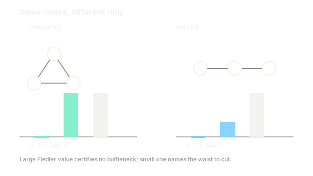
Triangle $K_3$ versus path $P_3$ , both on 3 nodes.

Adjacency: $K_3$ has $2, -1, -1$ (one large plus repeats from symmetry); $P_3$ has $\sqrt{2}, 0, -\sqrt{2} \approx 1.414, 0, -1.414$ . Radius $2$ versus $1.414$ : walks multiply faster on the triangle.

Laplacian: $K_3$ has $0, 3, 3$ (trace $6$ ); $P_3$ has $0, 1, 3$ (trace $4$ ). Fiedler values $3$ versus $1$ : the triangle resists cutting three times as hard, and indeed cutting $K_3$ in two severs 2 edges while $P_3$ needs 1. Cheeger reads the same story: large $\lambda_2$ certifies no bottleneck, small $\lambda_2$ names one.

Watch Out For

Hearing non-isomorphic drums as identical

Cospectral pairs (same Laplacian or adjacency spectrum, different graphs) exist past a handful of nodes: same eigenvalues, different cut structure, different dynamics details. A spectrum-only fingerprint collides.

Symptom: duplicate detection or anomaly flags miss obvious structural changes because eigenvalues barely move. Fix: pair spectra with local statistics (degree sequences, motif counts, walk profiles) and treat the spectrum as a strong filter, not a unique ID.

Rounding a gapless spectrum as if it were gapped

When $\lambda_3 - \lambda_2$ sits near zero, the Fiedler direction is one arbitrary rotation of a degenerate space: re-running the eigensolver returns a different "answer" for identical input, and clusters flip.

Symptom: partitions vary run to run while the spectrum barely changes. Fix: check the gap before cutting, stabilize with row-normalized multi-vector embeddings, or admit the graph has no clean two-way split at this scale.

The Quick Version

Adjacency spectra govern walk growth; Laplacian spectra govern cuts and cohesion.
Zero-count equals components; $\lambda_2$ prices the bottleneck both ways via Cheeger.
Triangle Laplacian $0, 3, 3$ dominates path $0, 1, 3$ : better knit, faster mixing, costlier cuts.
Fiedler rounding turns the continuous optimum into a real partition with guarantees.
Cospectral graphs share spectra but not shape; gapless spectra give unstable cuts.