Identifiability

A parameter is identifiable when different values leave different footprints in the data, so infinite observations could pin it down exactly.

An identifiable parameter gives each value its own likelihood peak, while a nonidentifiable pair shares a flat ridge where many values fit equally well

Why Does This Exist?

No estimator can recover what the data never recorded. If two parameter values generate identical data distributions, no sample size separates them: the likelihood ties forever, posteriors follow the prior along the tie, and reported standard errors mislead. Identifiability states this precondition before any estimation method runs.

The distinction that saves projects is structural versus practical. Structural nonidentifiability holds at infinite data (two values, same distribution, always). Practical nonidentifiability holds at your data: the values differ in principle but your sample is too small or noisy to tell. The first needs reparameterization; the second needs more or better data. Estimation methods like maximum likelihood assume the first is settled.

The one idea you need first

The map $\theta \mapsto P_\theta$ sends each parameter value to its data distribution. Identifiability means this map is injective (one-to-one): $\theta_1 \ne \theta_2$ implies $P_{\theta_1} \ne P_{\theta_2}$ . Everything below checks injectivity in concrete cases.

Think of It Like This

Two keys cut for the same lock

A locksmith cuts two different-looking keys and both turn your lock. From the lock's behavior alone you cannot tell which key was used: the mapping from key shape to turning outcome is not injective. No number of repeated turns separates them.

One fix changes the lock (reparameterization: combine the keys into the one cut that matters). The other changes the test (more data: try the keys in a second lock that distinguishes them). Structural failure is two keys for every lock of this type; practical failure is two keys for this particular worn lock only.

How It Actually Works

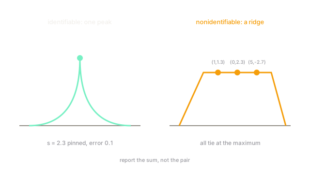
For data $X$ with family $\{P_\theta : \theta \in \Theta\}$ , $\theta$ is identifiable when the map is injective. A working test: the Fisher information at $\theta$ must be nonsingular. A singular information matrix means some direction changes nothing about the distribution to first order: a ridge, not a peak.

Canonical failures: (1) additive aliasing, $y = a + b + \text{noise}$ identifies only the sum $s = a + b$ , never the pair; (2) mixture label switching, swapping component labels leaves the mixture identical, so labels are unidentified without ordering constraints; (3) scale confounding, $y = \alpha \beta x$ identifies only the product. Canonical fix: estimate the identified combination ( $s$ , ordered components, the product) and report that.

Worked example

Model $y_i = a + b + \varepsilon_i$ with $\varepsilon_i$ standard normal, $n = 100$ observations, sample mean $\bar{y} = 2.3$ . The log-likelihood depends only on $s = a + b$ : $\ell = -\frac{n}{2}(\bar{y} - s)^2$ plus constants. Pairs $(a,b) = (1, 1.3)$ , $(0, 2.3)$ , $(5, -2.7)$ all give $\ell = 0$ (the maximum): a perfect ridge along $a + b = 2.3$ . The Fisher information matrix is all ones times $n$ , rank $1$ in $2$ dimensions, singular. The identified quantity $s$ has estimate $2.3 \pm 0.1$ (standard error $1/\sqrt{100}$ ); the pair $(a, b)$ has infinite uncertainty along the ridge no matter the $n$ .

Code

1def loglik(a: float, b: float, ybar: float = 2.3, n: int = 100) -> float:2    s = a + b  # only the sum enters the likelihood3    return -0.5 * n * (ybar - s) ** 24
5
6pairs = [(1.0, 1.3), (0.0, 2.3), (5.0, -2.7), (1.0, 1.0)]7for a, b in pairs:8    print(a, b, round(loglik(a, b), 1))9# -> 1.0 1.3 0.010# -> 0.0 2.3 0.011# -> 5.0 -2.7 0.012# -> 1.0 1.0 -4.5

The first three pairs tie at the maximum while $(1,1)$ trails by $4.5$ : a ridge, not a peak.

Watch Out For

Reporting software standard errors on a ridge

Optimizers stop somewhere along the ridge and report local curvature as certainty, producing tight intervals for values the data never pinned. Symptoms: estimates swing wildly across seeds while the loss barely moves. Diagnose with the information rank and profile likelihoods before publishing any interval.

Breaking symmetry with an arbitrary constraint and forgetting it

Fixing mixture labels by ordering means (e.g., $\mu_1 < \mu_2$ ) identifies the model but bakes the constraint into every conclusion. If the true components cross, the constraint silently biases. State the constraint alongside the estimate, and check the unconstrained posterior for a second mode the ordering hid.

The Quick Version

Identifiability means distinct parameters give distinct data distributions.
Structural failure persists at infinite data; practical failure yields to more or better data.
The Fisher information must be nonsingular; singular means a ridge.
In $y = a + b + \text{noise}$ with mean $2.3$ , the pairs $(1,1.3)$ , $(0,2.3)$ , $(5,-2.7)$ tie exactly.
Estimate identified combinations (sums, products, ordered components) and report those.
Never trust optimizer standard errors before checking the information rank.