Tensor Decomposition

Tensor decomposition breaks down high-dimensional arrays into products of simpler matrices and core tensors, exposing latent patterns while dramatically compressing parameters.

CP decomposition factors a 3D tensor into a sum of rank-one outer products, while Tucker decomposition compresses it into a small core tensor multiplied by factor matrices along each mode.

Why Does This Exist?

Machine learning models routinely process multidimensional data: video streams (frames $\times$ height $\times$ width $\times$ channels), recommendation logs (user $\times$ item $\times$ context $\times$ time), multi-relational knowledge graphs, and 4D convolutional weight filters. Storing and learning over raw multidimensional grids quickly triggers the curse of dimensionality — a fourth-order tensor with 100 entries per dimension requires $100^4 = 100,000,000$ floating-point parameters.

The naive workaround is flattening the tensor into a 2D matrix to apply standard linear algebra. Flattening, however, destroys the spatial and temporal correlations that span multiple modes simultaneously. It breaks multi-way interactions and forces matrix factorization algorithms to learn redundant parameters across unrolled indices.

Tensor decomposition provides the multilinear generalization of singular value decomposition and low-rank matrix approximation. By expressing high-order arrays as products of low-dimensional latent factor matrices and small core interaction tensors, tensor decomposition slashes parameter footprints from exponential $O(I^N)$ to linear $O(N \cdot I \cdot R)$ , separates multi-modal noise, and enables parameter-efficient neural network compression.

Think of It Like This

A 3D Lego sculpture vs. orthogonal profile ribbons

Imagine building a solid 3D sculpture inside a $100 \times 100 \times 100$ block grid. Storing the exact color and density of every individual voxel requires keeping track of $1,000,000$ distinct numbers.

Suppose, however, that the sculpture has coherent structural themes. Instead of cataloging every individual voxel in the cube, you capture three separate 1D ribbon profiles: a vertical profile across height, a horizontal profile across width, and a depth profile along thickness. Multiplying these three ribbons together paints an entire rank-one 3D block. By summing a modest collection of $R$ different ribbon sets, you rebuild the entire sculpture.

Instead of storing $1,000,000$ voxel entries, you store only $3 \times 100 \times R$ ribbon values. If $R = 10$ , that is just $3,000$ numbers — a $333\times$ reduction in storage with virtually no loss in structural clarity.

The analogy stops when data consists of unstructured white noise or highly irregular local spikes: true random high-dimensional noise cannot be separated into low-rank 1D ribbons without significant reconstruction error.

How It Actually Works

CP and Tucker Formulations

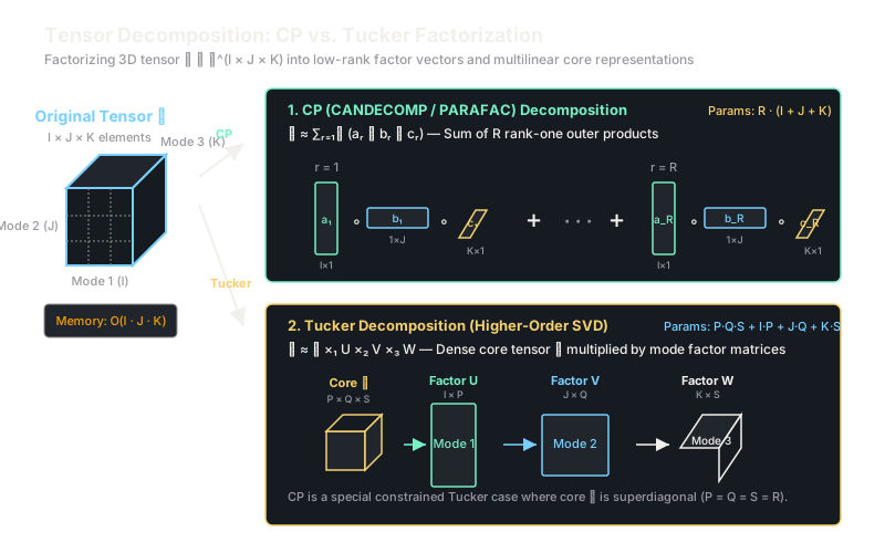
A tensor $\mathcal{X} \in \mathbb{R}^{I \times J \times K}$ is an order-3 multi-way array. The two foundational tensor decomposition families are CANDECOMP/PARAFAC (CP) and Tucker decomposition.

In CP decomposition, a tensor is approximated as a finite sum of $R$ rank-one tensors, where each rank-one component is an outer product $\circ$ of vectors:

\mathcal{X} \approx \sum_{r=1}^R \mathbf{a}_r \circ \mathbf{b}_r \circ \mathbf{c}_r

where $\mathbf{a}_r \in \mathbb{R}^I$ , $\mathbf{b}_r \in \mathbb{R}^J$ , and $\mathbf{c}_r \in \mathbb{R}^K$ . Stacking these vectors column-wise produces factor matrices $\mathbf{A} \in \mathbb{R}^{I \times R}$ , $\mathbf{B} \in \mathbb{R}^{J \times R}$ , and $\mathbf{C} \in \mathbb{R}^{K \times R}$ . For any individual coordinate $(i, j, k)$ :

\mathcal{X}_{ijk} \approx \sum_{r=1}^R A_{ir} B_{jr} C_{kr}

The smallest integer $R$ for which this equality holds exactly is the tensor rank. The parameter footprint collapses from $I \cdot J \cdot K$ down to $R(I + J + K)$ .

In Tucker decomposition (higher-order SVD), the factors are not forced to share a single rank $R$ . Instead, a small dense core tensor $\mathcal{G} \in \mathbb{R}^{P \times Q \times S}$ governs cross-mode interactions between orthogonal factor matrices $\mathbf{U} \in \mathbb{R}^{I \times P}$ , $\mathbf{V} \in \mathbb{R}^{J \times Q}$ , and $\mathbf{W} \in \mathbb{R}^{K \times S}$ :

\mathcal{X} \approx \mathcal{G} \times_1 \mathbf{U} \times_2 \mathbf{V} \times_3 \mathbf{W} = \sum_{p=1}^P \sum_{q=1}^Q \sum_{s=1}^S \mathcal{G}_{pqs} (\mathbf{u}_p \circ \mathbf{v}_q \circ \mathbf{w}_s)

where $\times_n$ denotes the mode- $n$ tensor-matrix product. CP decomposition is a constrained special case of Tucker where the core tensor $\mathcal{G}$ is strictly superdiagonal ( $P = Q = S = R$ with non-zero entries only when $p = q = s$ ).

To fit factor matrices from an observed tensor $\mathcal{X}$ , standard practice uses Alternating Least Squares (ALS). ALS fixes two factor matrices (e.g., $\mathbf{B}$ and $\mathbf{C}$ ) and solves a linear least squares regression for the third factor $\mathbf{A}$ using the Khatri-Rao product $\mathbf{C} \odot \mathbf{B}$ , cycling through all modes until convergence:

\mathbf{X}_{(1)} \approx \mathbf{A} (\mathbf{C} \odot \mathbf{B})^T \implies \mathbf{A} = \mathbf{X}_{(1)} \left[(\mathbf{C} \odot \mathbf{B})^T\right]^\dagger

where $\mathbf{X}_{(1)}$ is the mode-1 matrix unfolding of $\mathcal{X}$ , and $\dagger$ denotes the Moore-Penrose pseudoinverse.

Worked Example

Consider a $2 \times 2 \times 2$ third-order tensor $\mathcal{X}$ . We fit a rank-1 ( $R = 1$ ) CP decomposition defined by three factor vectors:

\mathbf{a} = \begin{bmatrix} 2 \\ 1 \end{bmatrix}, \quad \mathbf{b} = \begin{bmatrix} 3 \\ 4 \end{bmatrix}, \quad \mathbf{c} = \begin{bmatrix} 1 \\ 2 \end{bmatrix}

Let us compute the exact numerical reconstruction for all 8 elements using $\mathcal{X}_{ijk} = a_i \cdot b_j \cdot c_k$ :

Front slice ( $k = 0$ , where $c_0 = 1$ ):
- $\mathcal{X}_{0,0,0} = a_0 \cdot b_0 \cdot c_0 = 2 \times 3 \times 1 = 6$
- $\mathcal{X}_{0,1,0} = a_0 \cdot b_1 \cdot c_0 = 2 \times 4 \times 1 = 8$
- $\mathcal{X}_{1,0,0} = a_1 \cdot b_0 \cdot c_0 = 1 \times 3 \times 1 = 3$
- $\mathcal{X}_{1,1,0} = a_1 \cdot b_1 \cdot c_0 = 1 \times 4 \times 1 = 4$
Back slice ( $k = 1$ , where $c_1 = 2$ ):
- $\mathcal{X}_{0,0,1} = a_0 \cdot b_0 \cdot c_1 = 2 \times 3 \times 2 = 12$
- $\mathcal{X}_{0,1,1} = a_0 \cdot b_1 \cdot c_1 = 2 \times 4 \times 2 = 16$
- $\mathcal{X}_{1,0,1} = a_1 \cdot b_0 \cdot c_1 = 1 \times 3 \times 2 = 6$
- $\mathcal{X}_{1,1,1} = a_1 \cdot b_1 \cdot c_1 = 1 \times 4 \times 2 = 8$

Now consider an ALS step to solve for $\mathbf{a}$ given the observed slices and fixed factors $\mathbf{b}$ and $\mathbf{c}$ . The Khatri-Rao product $\mathbf{m} = \mathbf{c} \odot \mathbf{b}$ has elements: $m_0 = c_0 \cdot b_0 = 1 \times 3 = 3$ , $m_1 = c_0 \cdot b_1 = 1 \times 4 = 4$ , $m_2 = c_1 \cdot b_0 = 2 \times 3 = 6$ , $m_3 = c_1 \cdot b_1 = 2 \times 4 = 8$ . So $\mathbf{m} = [3, 4, 6, 8]^T$ .

Mode-1 unfolding $\mathbf{X}_{(1)}$ arranges row 0 as $[\mathcal{X}_{0,0,0}, \mathcal{X}_{0,1,0}, \mathcal{X}_{0,0,1}, \mathcal{X}_{0,1,1}] = [6, 8, 12, 16]$ . Notice that $[6, 8, 12, 16] = 2 \times [3, 4, 6, 8] = 2 \mathbf{m}^T$ . Row 1 is $[3, 4, 6, 8] = 1 \times [3, 4, 6, 8] = 1 \mathbf{m}^T$ . Solving $\mathbf{X}_{(1)} = \mathbf{a} \mathbf{m}^T$ recovers $\mathbf{a} = [2, 1]^T$ exactly.

Code

1import numpy as np2
3
4def cp_reconstruct_3d(5    factor_a: np.ndarray, factor_b: np.ndarray, factor_c: np.ndarray6) -> np.ndarray:7    """Reconstruct an order-3 tensor from CP factor matrices via outer products.8
9    Shapes:10        factor_a: (I, R)11        factor_b: (J, R)12        factor_c: (K, R)13    Returns:14        X: (I, J, K)15    """16    # einsum contracts mode factors along rank index r17    return np.einsum("ir,jr,kr->ijk", factor_a, factor_b, factor_c)18
19
20def khatri_rao(a: np.ndarray, b: np.ndarray) -> np.ndarray:21    """Column-wise Khatri-Rao product of two matrices."""22    r = a.shape[1]23    cols = [np.kron(a[:, col], b[:, col]) for col in range(r)]24    return np.column_stack(cols)25
26
27# Factor vectors for rank R=128a = np.array([[2.0], [1.0]])  # shape (2, 1)29b = np.array([[3.0], [4.0]])  # shape (2, 1)30c = np.array([[1.0], [2.0]])  # shape (2, 1)31
32tensor_x = cp_reconstruct_3d(a, b, c)33print(tensor_x.shape)34# -> (2, 2, 2)35
36print(tensor_x[:, :, 0])37# -> [[6. 8.]38# ->  [3. 4.]]39
40print(tensor_x[:, :, 1])41# -> [[12. 16.]42# ->  [ 6.  8.]]43
44# Unfold mode-1 and verify Khatri-Rao ALS recovery45x_mode1 = tensor_x.reshape(tensor_x.shape[0], -1)  # (2, 4)46kr_cb = khatri_rao(c, b)  # (4, 1)47a_recovered = x_mode1 @ kr_cb @ np.linalg.inv(kr_cb.T @ kr_cb)48
49print(np.allclose(a, a_recovered))50# -> True

Watch Out For

Tensor rank computation is NP-hard and rank approximations can be ill-posed

In matrix linear algebra, computing rank and finding the optimal low-rank matrix approximation is solved in polynomial time via SVD under the Eckart-Young-Mirsky theorem. For order-3 and higher tensors, computing tensor rank is proven to be NP-hard.

Even worse, the set of rank- $R$ tensors is not topologically closed for $R \ge 2$ . In iterative CP algorithms, this leads to the infamous "degeneracy problem": two or more rank-one components grow to massive magnitudes with opposing signs, attempting to cancel each other out while chasing an infimum that does not exist as a rank- $R$ tensor.

Fix: When fitting CP models, always impose $L_2$ regularisation on factor weights during Alternating Least Squares updates. If stable orthogonal decompositions are essential, choose Tucker decomposition or the Tensor Train (TT) format, whose truncation steps rely strictly on stable sequential SVD operations.

The Quick Version

CP decomposition factorizes an $N$ -way tensor into a sum of $R$ rank-1 vector outer products, reducing parameter count from $O(I^N)$ to $O(N \cdot I \cdot R)$ .
Tucker decomposition provides a multilinear SVD with orthogonal factor matrices along each mode governed by a dense core interaction tensor.
Unfolding multi-way tensors into matrices for standard SVD discards multilinear geometry and fails to capture higher-order dependencies.
Unlike matrix SVD, computing general tensor rank is NP-hard, and CP-ALS fitting requires norm regularization to avoid divergent degenerate components.
Modern deep networks use tensor decomposition (including Tensor Trains and Tucker) to compress multi-million parameter embedding layers and convolution weights.