Kernel Functions

A kernel tells you how alike two points are by returning their dot product in some big feature space, computed directly from the original coordinates without ever building that space.

Two inputs lift into a large feature space while the kernel shortcut returns 0.607 directly from the raw coordinates

Why Does This Exist?

Linear methods are fast but blind to curves: no straight line separates a ring from its center. Lifting points into a richer feature space fixes the blindness, yet the lifted coordinates can be infinite-dimensional, so building them is impossible. Kernel functions break the deadlock: algorithms like SVMs only ever need dot products between lifted points, and the kernel computes those from the raw inputs.

This page defines what makes a function a valid kernel and checks one on numbers. The algorithm that spends those dot products is the kernel trick; the space the lifting lands in is previewed in Hilbert spaces.

The one idea you need first

A positive definite matrix has all eigenvalues above zero, so every quadratic form through it stays nonnegative. Kernel validity is exactly this property demanded of every Gram matrix you can build. The matrix facts are in positive definite matrices.

Think of It Like This

A spice blend rated without tasting each spice

A chef rates how well two dishes pair without listing every molecule: one sniff of each finished plate gives a similarity score. The score behaves like a dot product of full ingredient lists, yet nobody wrote those lists down.

A kernel is that sniff. Two raw inputs go in, one similarity number comes out, and the number equals the inner product in a feature kitchen you never enter. Where it stops: not every similarity sniff qualifies. Only positive definite ones correspond to a real feature space; the rest silently produce nonsense geometry.

How It Actually Works

A function $k(x, z)$ is a kernel when it is symmetric and positive definite: for every finite set $x_1, \ldots, x_n$ , the Gram matrix $K_{ij} = k(x_i, x_j)$ is positive semidefinite ( $c^T K c \ge 0$ for all $c$ ). In plain words: $k$ returns a similarity, and no collection of points can force those similarities into a geometrically impossible shape.

Three kernels carry nearly all of practice. Linear: $k(x,z) = x^T z$ . Polynomial: $k(x,z) = (x^T z + c)^d$ . Gaussian RBF: $k(x,z) = \exp(-\|x-z\|^2 / 2\sigma^2)$ with width $\sigma$ . Mercer's theorem says each valid kernel is genuinely a dot product $k(x,z) = \langle \phi(x), \phi(z) \rangle$ in some Hilbert space, and the RBF's space is infinite-dimensional.

Worked example

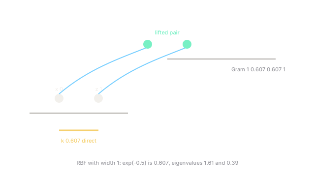
Take the RBF kernel with $\sigma = 1$ on points $x = 0$ and $z = 1$ . Then $\|x - z\|^2 = 1$ , so $k(0,1) = \exp(-1/2) \approx 0.607$ . Diagonal entries are $k(0,0) = k(1,1) = 1$ , giving Gram matrix:

K = \begin{bmatrix} 1 & 0.607 \\ 0.607 & 1 \end{bmatrix}

Eigenvalues: $1 + 0.607 = 1.607$ and $1 - 0.607 = 0.393$ . Both positive, so $K$ is positive definite and this kernel behaves like a genuine dot product here. Small width pushes $0.607$ toward $0$ (near-orthogonal); large width pushes it toward $1$ (near-identical).

Code

Build the Gram matrix and check its eigenvalues stay positive, the validity test for any kernel.

1import numpy as np2
3
4def rbf_gram(xs: np.ndarray, sigma: float = 1.0) -> np.ndarray:5    d2 = (xs[:, None] - xs[None, :]) ** 2  # pairwise squared distances6    return np.exp(-d2 / (2 * sigma**2))  # RBF similarity7
8
9xs = np.array([0.0, 1.0])10print(rbf_gram(xs))  # -> [[1. 0.607] [0.607 1.]]11print(np.linalg.eigvalsh(rbf_gram(xs)))  # -> [0.393 1.607]

Ones on the diagonal, $0.607$ off it, eigenvalues $0.39$ and $1.61$ : positive, exactly as computed by hand.

Watch Out For

Inventing a similarity that is not positive definite

Symptom: a custom kernel trains fine on small data then yields indefinite Gram matrices (negative eigenvalues like $-0.3$ ) and the optimizer oscillates. Fix: eigencheck every new kernel on a few hundred points first; build custom kernels only from sums, products and scalings of known-valid ones.

Setting the RBF width by gut feeling

Symptom: tiny $\sigma$ makes every Gram entry off-diagonal $\approx 0$ (memorization), huge $\sigma$ makes them all $\approx 1$ (underfit). Fix: grid-search $\sigma$ against validation error, or start from the median pairwise distance heuristic and tune from there.

The Quick Version

A kernel returns the dot product in a feature space you never construct.
Validity means every Gram matrix is positive semidefinite, checked through eigenvalues.
Linear, polynomial and RBF kernels cover nearly all practice; RBF's feature space is infinite-dimensional.
Points $0$ and $1$ with unit width score $0.607$ , with Gram eigenvalues $1.61$ and $0.39$ .
Width controls similarity scale: small widths orthogonalize, large widths merge.