Poisson Processes

A model for arrivals that come one at a time, at a steady average rate, with no memory and no bunching built in. Clicks, calls, decays and goals.

Arrivals at rate 3 per hour land as isolated ticks with uneven gaps, and the count in any hour follows the Poisson probabilities 0.05, 0.15, 0.22 and 0.22

Why Does This Exist?

Many ML inputs are event streams: ad clicks, support tickets, server errors, sensor triggers. The Poisson process is the default model for such streams when events arrive singly at a steady average rate with no aftereffects. It gives closed forms for everything you need: the count in any window, the wait until the next event, and the likelihood of an observed stream, which is what lets you fit the rate from data.

It also sits underneath half of applied probability. The number of arrivals in a window of length $t$ at rate $\lambda$ is Poisson with mean $\lambda t$ . The gaps between arrivals are independent exponentials with mean $1/\lambda$ . And the central limit theorem eventually describes the count when the rate is large. This page covers the process itself; the distribution family is in probability distributions.

The one idea you need first

A Poisson random variable with mean $\mu$ takes values $k = 0, 1, 2, \ldots$ with $P(K = k) = e^{-\mu}\mu^k / k!$ . Mean equals variance equals $\mu$ . That single equality is also the diagnostic: real streams whose variance far exceeds the mean are overdispersed and need a richer model.

Think of It Like This

Popcorn in a steady microwave

Kernels pop one at a time at a roughly steady pace. Knowing that nothing popped in the last ten seconds tells you nothing about the next ten: no kernel remembers, none is due. Sometimes two pops land close together by pure chance, and that clump means nothing.

The rate knob is the power setting. Turn it up and pops come faster on average, but each individual gap stays unpredictable. The Poisson process is this picture with the mathematics filled in: rate $\lambda$ is the power setting, the exponential gap is the unpredictability of each wait, and the Poisson count is how many pops a timed window catches.

Where the analogy stops: real popcorn changes rate as kernels deplete. The basic Poisson process holds $\lambda$ fixed; a rate that varies with time needs the nonhomogeneous version.

How It Actually Works

A homogeneous Poisson process with rate $\lambda$ satisfies three axioms: counts in disjoint windows are independent, the distribution in a window depends only on its length, and two arrivals never land at exactly the same instant. From these, the count $N(t)$ in a window of length $t$ is Poisson with mean $\lambda t$ :

P(N(t) = k) = \frac{e^{-\lambda t}(\lambda t)^k}{k!}

The gap $T$ between consecutive arrivals is exponential with density $\lambda e^{-\lambda t}$ and mean $1/\lambda$ , and it is memoryless: $P(T > s + t \mid T > s) = P(T > t)$ . This is why the process never gets due for an arrival.

Worked example

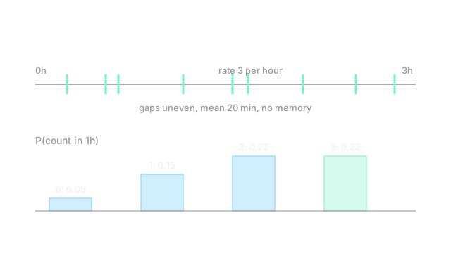
Support tickets arrive at $\lambda = 3$ per hour. For a one-hour window, $\mu = 3$ :

$P(N = 0) = e^{-3} \approx 0.0498$ , about 5 percent of hours are silent.
$P(N = 1) = 3e^{-3} \approx 0.149$ , about 15 percent.
$P(N = 2) = 9e^{-3}/2 \approx 0.224$ , about 22 percent.
$P(N = 3) = 27e^{-3}/6 \approx 0.224$ , about 22 percent.

The chance of more than 5 arrivals is $1 - e^{-3}(1 + 3 + 4.5 + 4.5 + 3.375 + 2.025) \approx 1 - 0.916 = 0.084$ . Mean gap between tickets is $1/3$ hour, 20 minutes, but the chance a gap exceeds 40 minutes is $e^{-3 \times 2/3} = e^{-2} \approx 0.135$ .

Fitting the rate is one line: observe $n$ arrivals over total time $T$ and $\hat{\lambda} = n/T$ . Ten tickets in four hours gives $\hat{\lambda} = 2.5$ per hour.

Code

This checks the worked probabilities and the memoryless gap property by direct simulation.

1import numpy as np2
3rng = np.random.default_rng(3)4lam = 3.0  # arrivals per hour5gaps = rng.exponential(1 / lam, size=20000)  # mean gap 20 minutes6print(round(float(np.mean(gaps)), 3))  # -> 0.333 hours7print(round(float(np.mean(gaps > 2 / 3)), 3))  # -> 0.1358counts = rng.poisson(lam, size=20000)  # arrivals per hour9print(round(float(np.mean(counts == 0)), 3))  # -> 0.05

The three prints land near 0.333, 0.135 and 0.05, matching $1/3$ hours, $e^{-2}$ and $e^{-3}$ . If your stream's sample variance is triple its mean, stop here and reach for a negative-binomial or Hawkes model instead.

Watch Out For

Fitting Poisson to bursty data

Real arrivals often come in bursts: one outage triggers fifty alerts in a minute. The Poisson variance-equals-mean check catches this immediately. On bursty data the Poisson fit underestimates both silence and storms, so capacity planned from it fails exactly when load spikes. Test dispersion first; use a Hawkes self-exciting process when an arrival raises the near-term rate.

Assuming the rate is constant across the day

Ticket arrivals at 3 per hour on average might be 8 per hour at noon and 0.2 at night. A homogeneous fit averages these into a rate that describes no actual hour, and staffing from it leaves noon drowning and midnight overstaffed. Segment by hour or fit a nonhomogeneous $\lambda(t)$ before trusting any probability the model quotes.

The Quick Version

A Poisson process models single arrivals at a steady rate with no memory.
Counts in a window of length $t$ are Poisson with mean $\lambda t$ ; gaps are exponential with mean $1/\lambda$ .
At rate 3 per hour, silent hours happen about 5 percent of the time and the mean gap is 20 minutes.
The rate estimate is arrivals divided by total time: 10 tickets in 4 hours means 2.5 per hour.
Variance far above the mean means the data is overdispersed, so use a richer model.
A rate that drifts with time of day needs segmenting or a nonhomogeneous process.