Theory of Deep Learning

Why Does This Exist?

Neural networks beat older methods on images, speech, and language, yet for years nobody could say why depth helped or when training would succeed. Practitioners stacked layers because it worked; skeptics pointed out that the training problem is non-convex and the models have more parameters than data points, which classical statistics calls a mistake.

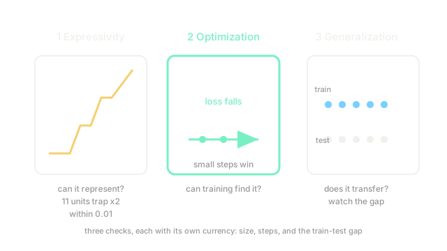
The theory exists to split that puzzle into three questions you can answer separately. Expressivity: which functions can a network of a given size represent? Optimization: why does a simple gradient method find good parameters on a non-convex surface? Generalization: why do those parameters predict on fresh data instead of memorizing? Each pillar has its own results, and each is covered by its own page: universal approximation, depth versus width, the loss surface, and over-parameterized generalization.

This page is the map, not the territory. It states the three questions, shows how they connect, and names what each one costs.

The one idea you need first

A network with one hidden layer computes sums of bent lines: each hidden unit applies a nonlinearity such as ReLU to a weighted sum, and the output adds those up. Everything in this page follows from asking what sums of bent pieces can build, how gradient steps adjust the bends, and why the result transfers to new inputs.

Think of It Like This

How It Actually Works

The three pillars, each in one paragraph with its key quantity:

1. Expressivity asks what functions a network can approximate and at what size. The classic answer is that one wide hidden layer approximates any continuous function on a compact set, and the modern answer is that depth builds the same functions with far fewer units for structured targets. The currency is parameter count versus approximation error.

2. Optimization asks why gradient descent trains a non-convex model at all. Part of the answer is over-parameterization: with more parameters than needed, the surface near initialization behaves almost linearly, so small steps keep making progress instead of stalling at bad saddles. The currency is the loss value over training steps.

3. Generalization asks why the trained net predicts on new inputs. Classical bounds based on parameter counts are vacuous here (they predict nothing), so the real answers track implicit preferences of the optimizer: among all settings that fit training data, gradient methods land on simple ones with small norms or large margins. The currency is the gap between train and test error.

How the three connect

Expressivity without optimization is a catalog of functions you cannot reach. Optimization without generalization is memorization machinery. The connection practitioners use daily: pick depth for structure (pillar 1), train with small steps from a careful start (pillar 2), and watch held-out error rather than parameter counts (pillar 3). When a model fails, the pillars localize the fault: underfitting points at pillar 1, stalled training at pillar 2, and a wide train-test gap at pillar 3.

Worked example

A concrete sense of scale for pillar 1. Approximate $f(x) = x^2$ on $[-1, 1]$ with ReLU pieces to error below $0.01$ in the maximum norm. A piecewise-linear fit with $k$ equal segments has error about $1/k^2$ (each segment of width $2/k$ deviates at most $(1/k)^2$ from the parabola). Setting $1/k^2 < 0.01$ gives $k > 10$, so about $11$ hidden units suffice, each unit placing one kink. That is expressivity as bookkeeping: error target in, unit count out. Pillars 2 and 3 then ask whether training finds those $11$ kinks and whether they sit in the right places for points between the training samples.

Code

This snippet counts the kinks a one-hidden-layer ReLU net can place, which is the raw material of expressivity arguments:

1def max_kinks(n_hidden: int) -> int:2    return n_hidden  # one ReLU unit places at most one kink on the line3
4
5def segments(n_hidden: int) -> int:6    return max_kinks(n_hidden) + 1  # kinks cut the line into pieces7
8
9for n in (2, 5, 11, 50):10    print(n, segments(n))  # -> 2 3, 5 6, 11 12, 50 51

Eleven units give twelve linear pieces, matching the hand count above: enough pieces to trap $x^2$ within $0.01$ on $[-1, 1]$.

Watch Out For

The Quick Version

• Deep learning theory asks three separate questions: what nets can represent, why training finds it, and why it predicts on new data.
• Expressivity trades parameter count against approximation error, and depth spends that budget better than width on structured targets.
• Optimization works partly because over-parameterization keeps the surface near initialization almost linear.
• Generalization in big models comes from the optimizer's preference for simple fits, not from having few parameters.
• Diagnose failures by pillar: underfitting, stalled training, and train-test gaps each point at a different one.
• Eleven ReLU units trap $x^2$ within $0.01$ on $[-1, 1]$, since piecewise error falls like $1/k^2$.

What to Read Next

• Convexity and Loss Landscapes
• Computational Complexity for ML