Physical AI: From Perception to Action

Physical AI closes the loop between sensors, computation, and motors in the real world. Unlike software models that generate static answers, physical agents must act against latency, continuous contact dynamics, and irreversible inertia.

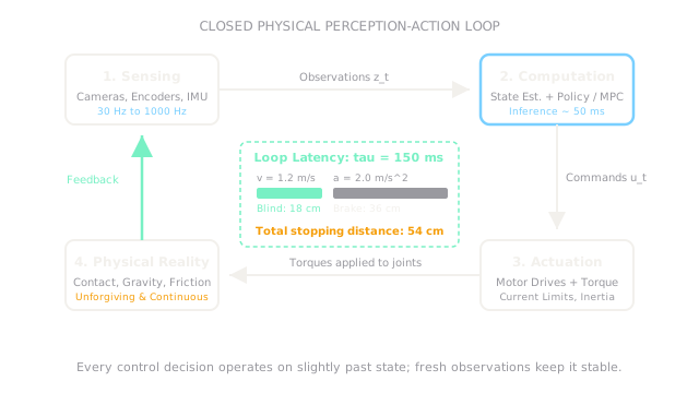
Physical AI closes the perception-action loop against real-world latency, where a 150 ms sensing delay produces 18 cm of blind motion

Why Does This Exist?

In pure software, an artificial intelligence model takes an input query, processes it through neural weights, and returns text, an image, or a class score. If the server stalls for two seconds, the user waits. The world does not crash.

In physical reality, that assumption dissolves immediately. When a 50 kg mobile delivery base rolls across concrete at $1.2\text{ m/s}$ , the ground pushes back with friction, wheels slip on dust, and obstacles move unexpectedly. If your perception stack takes 150 milliseconds to process a camera frame and issue a braking command, the robot travels nearly 20 centimeters before its brakes even engage.

Physical AI is the discipline of closing the perception-action loop reliably across real time, unmodeled physical contact, and sensor noise. It is broader than training neural policies with reinforcement learning: it encompasses sensor calibration, coordinate transformations, feedback controllers, state estimators, and safety shields. The core idea that separates it from standard digital AI is that physical actions have irreversible consequences.

Basics first: the learning side of physical embodiment lives in embodied-ai. How individual sensors, motors, and processors work together lives in robot-anatomy. The low-level correction loops that keep motion stable live in robot-feedback-control.

Think of It Like This

Driving on ice with a laggy windshield heads-up display

Imagine driving an electric car on a winding icy road at dusk. Instead of looking directly through the clear glass, you must steer using a digital display that updates with a slight video lag: every image you see happened 150 milliseconds ago.

You tap the brake pedal, but the icy road means deceleration is capped. If you steer assuming the car is already where the screen shows it, you overcorrect and spin out. To stay in your lane, you cannot treat the video feed as the present truth. You must maintain a running mental estimate of your actual current position, anticipate how the car's physical mass slides forward during the delay, and steer ahead of the lag.

Where it stops: human drivers have instinctive inner-ear vestibular balance and tactile feedback through their hands on the steering wheel. A physical AI robot has no innate intuition of balance or momentum—every millisecond of delay, sensor bias, and motor saturation must be explicitly modeled, estimated, and controlled in software and hardware.

How It Actually Works

The closed perception-action loop

Physical AI structures machine intelligence into four continuous, coupled stages operating at distinct rates:

Sensing: Proprioceptive sensors (encoders, IMUs, current sensors) measure internal machine state at high frequencies ( $500\text{ Hz}$ to $1000\text{ Hz}$ ). Exteroceptive sensors (RGB cameras, LiDAR, depth sensors) measure external environment geometry at lower frequencies ( $10\text{ Hz}$ to $60\text{ Hz}$ ).
State Estimation: Combines noisy raw measurements with a predictive motion model to estimate true robot pose $\mathbf{x}_t$ and world obstacles.
Planning and Policy: High-level trajectory planners or learned neural policies compute target waypoints, joint positions, or end-effector wrenches to achieve an objective.
Actuation and Control: Motor drives convert commanded setpoints into physical currents and torques $\boldsymbol{\tau}_t$ delivered to brushless motors and gearboxes.

The cost of real-world latency

Let a mobile robot travel at forward velocity $v$ toward a detected obstacle. The total loop latency $\tau_{\text{loop}}$ includes:

\tau_{\text{loop}} = \tau_{\text{exposure}} + \tau_{\text{transport}} + \tau_{\text{inference}} + \tau_{\text{actuator}}

where $\tau_{\text{exposure}}$ is the camera shutter time, $\tau_{\text{transport}}$ is the communication bus delay across CAN bus or Ethernet, $\tau_{\text{inference}}$ is the neural network or optimizer evaluation time, and $\tau_{\text{actuator}}$ is the physical current rise time in the motor windings.

During this delay $\tau_{\text{loop}}$ , the robot executes whatever command was issued previously. The blind unmonitored displacement $d_{\text{blind}}$ is:

d_{\text{blind}} = v \times \tau_{\text{loop}}

Once braking torque engages, the vehicle decelerates at maximum acceleration $a_{\text{brake}}$ governed by tire friction. The physical braking distance $d_{\text{brake}}$ is:

d_{\text{brake}} = \frac{v^2}{2 a_{\text{brake}}}

Total stopping distance required to prevent collision is:

d_{\text{total}} = d_{\text{blind}} + d_{\text{brake}} = v \tau_{\text{loop}} + \frac{v^2}{2 a_{\text{brake}}}

Worked example: a tabletop mobile base

Consider a mobile robot moving at speed $v = 1.2\text{ m/s}$ in a shared warehouse aisle.

Sensing, inference, and communication latency: $\tau_{\text{loop}} = 150\text{ ms} = 0.15\text{ s}$ .
Emergency braking deceleration limit: $a_{\text{brake}} = 2.0\text{ m/s}^2$ .

Compute the blind displacement during delay:

d_{\text{blind}} = 1.2 \times 0.15 = 0.18\text{ m} = 18\text{ cm}

Compute the physical braking distance:

d_{\text{brake}} = \frac{1.2^2}{2 \times 2.0} = \frac{1.44}{4.0} = 0.36\text{ m} = 36\text{ cm}

Total stopping distance:

d_{\text{total}} = 0.18 + 0.36 = 0.54\text{ m} = 54\text{ cm}

If an obstacle is detected at a distance of $0.40\text{ m}$ ( $40\text{ cm}$ ), open-loop or delayed execution results in an unavoidable collision: the robot travels $18\text{ cm}$ before slowing down, leaving only $22\text{ cm}$ of clearance where $36\text{ cm}$ was physically required.

Code

This standalone snippet verifies the stopping distance calculation and tests whether candidate sensor latencies maintain a required safety margin.

1def calculate_stopping_distance(2    velocity_mps: float,3    latency_sec: float,4    decel_mps2: float,5) -> tuple[float, float, float]:6    """Compute blind delay displacement, braking distance, and total stopping distance."""7    d_blind: float = velocity_mps * latency_sec8    d_brake: float = (velocity_mps ** 2) / (2.0 * decel_mps2)9    d_total: float = d_blind + d_brake10    return round(d_blind, 3), round(d_brake, 3), round(d_total, 3)11
12
13# Baseline scenario: 1.2 m/s, 150 ms latency, 2.0 m/s^2 brake deceleration14blind, brake, total = calculate_stopping_distance(1.2, 0.15, 2.0)15print(blind)  # -> 0.1816print(brake)  # -> 0.3617print(total)  # -> 0.5418
19# Check safety for an obstacle detected at 0.40 m clearance20clearance_m: float = 0.4021is_safe: bool = total <= clearance_m22print(is_safe)  # -> False

Watch Out For

Assuming zero-delay execution in software simulations

The most common failure in Physical AI is developing policies or planners in simulated environments that evaluate instantaneously. In simulation, an action chosen at step $t$ applies to physics at step $t$ . On physical hardware, processing a high-resolution camera image through a vision-language model can take 100 to 200 ms.

The symptom is severe tracking oscillation, overshoot, or outright collision when deploying a simulation-trained policy to hardware. Fix it by explicitly measuring hardware pipeline latency and buffering historical states, or by training policies with randomized observation delays that mirror the real compute hardware.

Treating high-level goal success as physical safety certification

A policy or model that scores 98% success on a pick-and-place task in clean laboratory conditions is not safe for deployment around people. High-level policies optimize task reward or imitation loss, but cannot guarantee torque limits, thermal dissipation, or boundary constraints under unexpected sensor dropouts.

The symptom is an autonomous arm that suddenly jerks at maximum torque when an object is slightly occluded. Fix it by separating high-level learned policies from independent, deterministically certified low-level safety shields: hardware watchdog timers, Cartesian velocity clamps, and joint torque limits that override model commands whenever safe operational bounds are exceeded (explored in physical AI safety and reliability).

The Quick Version

Physical AI closes the perception-action loop between sensory measurement, numerical decision-making, and physical motor actuation in the real world.
Real-world interaction is fundamentally constrained by latency, unmodeled contact mechanics, friction, and irreversible physical momentum.
Sensing-to-actuation delay produces blind displacement: at $1.2\text{ m/s}$ with $150\text{ ms}$ latency, a robot travels $18\text{ cm}$ before motor braking begins.
Multi-rate compute architectures split responsibilities: high-frequency real-time microcontrollers handle fast motor reflexes ( $1\text{ kHz}$ ), while onboard GPUs run perceptual models and policies ( $10\text{ Hz}$ to $50\text{ Hz}$ ).
Reliable physical systems rely on defense-in-depth: learned policies propose actions, but independent low-level safety clamps and hardware watchdogs enforce physical limits.