Feedback Control and PID

Open-loop commands fail when real friction, inertia, and payload variations oppose motion. Feedback control continuously compares desired target states to sensor measurements, issuing corrective commands through proportional, integral, and derivative terms.

Feedback control compares target setpoint to measured joint angle, computing P, I, and D torque commands

Why Does This Exist?

In idealized software, if you want a robotic joint to rotate to $45^\circ$ , you might simply command motor voltage for the time it theoretically takes to get there. In physical reality, open-loop control fails immediately: bearing friction resists rotation, a heavy tool payload changes the link's inertia, motor windings heat up and alter internal resistance, and external bumps knock the arm off course.

Feedback control continuously observes what the robot is actually doing and adjusts the commanded control signal to eliminate the difference.

The Proportional-Integral-Derivative (PID) controller is the workhorse reflex of physical robotics. It provides the low-level closed-loop stability that keeps joint motors locked onto planned trajectories despite real-world disturbances.

Basics first: the sensors and motor drives that execute these feedback loops live in robot-anatomy. Mapping Cartesian trajectories into joint setpoints lives in robot-forward-inverse-kinematics. Optimizing control commands over future predictive horizons lives in robot-model-predictive-control.

Think of It Like This

Driving a car at a constant speed up a steep mountain highway

Imagine setting your car's cruise control to 65 miles per hour on a flat highway, then beginning a steep uphill climb.

Proportional (P): As soon as your speed drops to 62 mph (a 3 mph error), you press the gas pedal down proportional to that deficit. But on a steep hill, a fixed pedal position only balances gravity at 63 mph—you remain permanently 2 mph below your setpoint (steady-state error).
Integral (I): You notice that you have been stuck below 65 mph for several seconds. The integral term accumulates that persistent past deficit and pushes the pedal deeper and deeper until the car finally reaches exactly 65 mph.
Derivative (D): As you crest the hill and your speed accelerates rapidly toward 65 mph, the derivative term detects the high rate of change and eases off the gas early to prevent surging over the speed limit.

Where it stops: human drivers can see the steep hill ahead and step on the gas before the car slows down (feedforward control). A standard PID controller is purely reactive: it cannot produce any corrective torque until an error has already appeared in the encoder readings.

How It Actually Works

The continuous and discrete PID formulation

Given a desired reference setpoint $r(t)$ (such as a joint angle target) and a measured output $y(t)$ , the tracking error $e(t)$ is:

e(t) = r(t) - y(t)

The continuous PID control law computes commanded torque $u(t)$ :

u(t) = K_p e(t) + K_i \int_0^t e(\tau) d\tau + K_d \frac{de(t)}{dt}

where:

$K_p$ (Proportional gain): Reacts to current error. Higher $K_p$ increases responsiveness and stiffness, but excessive $K_p$ induces oscillations and instability.
$K_i$ (Integral gain): Accumulates persistent past errors to eliminate steady-state offset caused by constant gravity or Coulomb friction.
$K_d$ (Derivative gain): Predicts future error by measuring rate of change, providing synthetic damping that suppresses overshoot.

On digital microcontrollers running at discrete sampling interval $\Delta t$ , the controller evaluates at discrete step $k$ :

e_k = r_k - y_k

I_k = I_{k-1} + e_k \Delta t

D_k = \frac{e_k - e_{k-1}}{\Delta t}

u_k = K_p e_k + K_i I_k + K_d D_k

Actuator limits and saturation clamping

Every physical electric motor has hard current and torque limits governed by magnetic saturation and thermal dissipation:

u_{\text{clamped}} = \text{clip}(u_k, -u_{\max}, +u_{\max})

If the integrator continues accumulating error while the actuator is clamped at $u_{\max}$ (for instance, when an arm pushes against an immovable physical barrier), the integral term grows to a massive value. When the barrier is removed, the stored integral holds the motor at maximum torque for seconds, causing massive overshoot. This dangerous phenomenon is integral windup, prevented by anti-windup clamping.

Worked example: joint position error correction

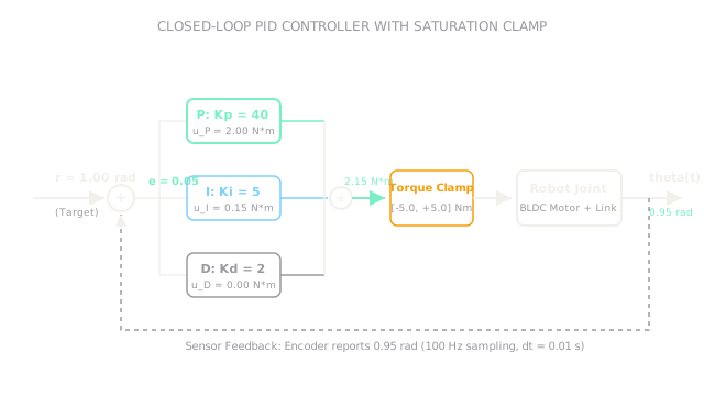
Consider an industrial robot joint position loop running at $100\text{ Hz}$ ( $\Delta t = 0.01\text{ s}$ ):

Target setpoint: $r_k = 1.00\text{ rad}$ .
Measured encoder position: $y_k = 0.95\text{ rad}$ .
Tracking error: $e_k = 1.00 - 0.95 = 0.05\text{ rad}$ .
Steady prior error: $e_{k-1} = 0.05\text{ rad}$ .
Accumulated integral state before this step: $I_{k-1} = 0.0295\text{ rad}\cdot\text{s}$ .
Controller gains:
- $K_p = 40.0\text{ N}\cdot\text{m/rad}$
- $K_i = 5.0\text{ N}\cdot\text{m/(rad}\cdot\text{s)}$
- $K_d = 2.0\text{ N}\cdot\text{m/(rad/s)}$

First, update the integral accumulator:

I_k = I_{k-1} + e_k \Delta t = 0.0295 + 0.05(0.01) = 0.0295 + 0.0005 = 0.0300\text{ rad}\cdot\text{s}

Second, compute the discrete error derivative:

D_k = \frac{e_k - e_{k-1}}{\Delta t} = \frac{0.05 - 0.05}{0.01} = 0.0\text{ rad/s}

Third, compute each term's contribution:

u_P = K_p e_k = 40.0 \times 0.05 = 2.00\text{ N}\cdot\text{m}

u_I = K_i I_k = 5.0 \times 0.0300 = 0.15\text{ N}\cdot\text{m}

u_D = K_d D_k = 2.0 \times 0.0 = 0.00\text{ N}\cdot\text{m}

Sum the terms to find total commanded motor torque:

u_k = u_P + u_I + u_D = 2.00 + 0.15 + 0.00 = 2.15\text{ N}\cdot\text{m}

The motor driver receives a torque command of $2.15\text{ N}\cdot\text{m}$ . Since this falls comfortably within the actuator's $\pm 5.0\text{ N}\cdot\text{m}$ torque saturation clamp, the full torque is delivered to the motor phase windings to accelerate the joint toward $1.00\text{ rad}$ .

Code

This Python snippet implements a complete discrete PID controller class with output torque clamping and integral anti-windup protection.

1class DiscretePID:2    def __init__(3        self,4        kp: float,5        ki: float,6        kd: float,7        dt: float,8        u_max: float,9    ) -> None:10        self.kp = kp11        self.ki = ki12        self.kd = kd13        self.dt = dt14        self.u_max = u_max15        self.integral: float = 0.016        self.prev_error: float = 0.017
18    def update(self, target: float, measured: float) -> tuple[float, float, float, float]:19        error: float = target - measured20
21        # Anti-windup: only integrate if output is not saturated22        self.integral += error * self.dt23        derivative: float = (error - self.prev_error) / self.dt24        self.prev_error = error25
26        u_p: float = self.kp * error27        u_i: float = self.ki * self.integral28        u_d: float = self.kd * derivative29        u_raw: float = u_p + u_i + u_d30
31        # Clamping32        u_clamped: float = max(-self.u_max, min(self.u_max, u_raw))33        return round(u_p, 3), round(u_i, 3), round(u_d, 3), round(u_clamped, 3)34
35
36# Initialize PID controller with Kp=40, Ki=5, Kd=2, dt=0.01s, max torque 5.0 Nm37pid = DiscretePID(kp=40.0, ki=5.0, kd=2.0, dt=0.01, u_max=5.0)38
39# Simulate prior step to prime state40pid.integral = 0.029541pid.prev_error = 0.0542
43up, ui, ud, u_total = pid.update(target=1.00, measured=0.95)44print(up)       # -> 2.045print(ui)       # -> 0.1546print(ud)       # -> 0.047print(u_total)  # -> 2.15

Watch Out For

Unfiltered derivative kick on noisy encoder signals

Calculating derivative $D_k = (e_k - e_{k-1}) / \Delta t$ directly from discrete encoder counts amplifies electronic quantization noise. When $\Delta t = 1\text{ ms}$ , a single encoder count fluctuation turns into hundreds of rad/s $^2$ of apparent acceleration.

The symptom is high-frequency buzzing, rapid heating of the motor casing, and violent acoustic chattering even when the arm is standing still. Fix it by computing the derivative directly from filtered joint velocity sensors (such as tachometers or state estimators), or passing the derivative term through a first-order low-pass filter: $D_{\text{filtered}} = \alpha D_k + (1-\alpha) D_{\text{filtered}}$ .

Integral windup during motor saturation or mechanical contact

When a robotic arm reaches down to pick up an object and encounters unexpected contact, the error cannot reach zero. The integral term continues accumulating error for hundreds of cycles, saturating the controller.

The symptom is that when the arm finally lifts off the surface, it violently launches upward at maximum acceleration as the oversized integral discharges. Fix it by implementing back-calculation or conditional integration (clamping the integral accumulation whenever commanded output $u_k$ exceeds actuator saturation bounds).

The Quick Version

Feedback control continuously measures joint positions to compute real-time corrective torques against real friction, gravity, and inertia.
The PID controller combines present error (Proportional), accumulated past error (Integral), and predicted rate of change (Derivative).
At $\Delta t = 0.01\text{ s}$ with $K_p = 40, K_i = 5, K_d = 2$ , an error of $0.05\text{ rad}$ produces a commanded motor torque of $2.15\text{ N}\cdot\text{m}$ .
Integral action eliminates steady-state droop caused by gravity, but must be protected against integral windup during torque saturation.
Pure numerical differentiation amplifies high-frequency encoder noise into motor chatter; robust controllers filter velocity signals before derivative computation.