Robot Anatomy: Sensors, Actuators and Compute

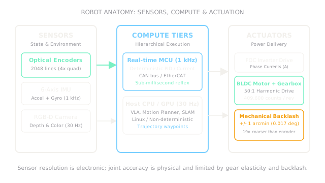
Robots bridge software to physical reality through three distinct subsystems: proprioceptive and exteroceptive sensors that measure physical state, actuators that deliver mechanical power, and hierarchical compute running real-time control alongside neural policies.

Robot anatomy links sensors, multi-tier compute, and actuators, where a 50:1 gearbox yields 409,600 counts per joint revolution

Why Does This Exist?

In high-level AI literature, an agent is often treated as a mathematical abstraction: state in, action out. But on real hardware, an action cannot simply be "move forward 10 centimeters." A motor controller does not accept Cartesian distance; it accepts pulse-width modulation duties, phase currents, or target velocity setpoints.

Without understanding robot anatomy, software engineers make two costly mistakes: they assume sensors report truth without noise or bias, and they assume actuators reach commanded positions instantaneously with zero error.

Robot anatomy breaks down the physical machine into three interacting subsystems:

Sensors that convert physical quantities into discrete electronic numbers.
Compute hardware structured into strict real-time reflex loops and high-level reasoning tiers.
Actuators and transmissions that convert electrical energy into mechanical torque while battling backlash, friction, and thermal dissipation.

Basics first: the overall loop lives in physical-ai-overview. How multiple joints combine into coordinate spaces lives in robot-degrees-of-freedom. Turning raw camera pixels into spatial coordinates lives in robot-perception-geometry.

Think of It Like This

The human nervous system: spinal cord reflexes versus cerebral cortex planning

Think of how your own body catches a falling coffee mug. Your eyes perceive the cup slipping (exteroceptive sensing), while stretch receptors in your tendons and muscle spindles report arm joint angles (proprioception).

When your fingertip touches the ceramic, a $1000\text{ Hz}$ reflex loop inside your spinal cord immediately fires motor neurons to grip tighter before the signal even reaches your conscious brain. Meanwhile, your cerebral cortex runs at a much slower deliberative rate ( $10\text{ Hz}$ to $20\text{ Hz}$ ), deciding whether to set the mug on the table or yell for a napkin.

Where it stops: biological muscles pull via contracting actin-myosin fibers in opposing pairs (biceps and triceps), and tendons provide soft non-linear elasticity. Robots use bidirectional electric brushless motors and rigid steel or strain-wave gearboxes, where mechanical play (backlash) and thermal resistance govern motor limits rather than muscle fatigue.

How It Actually Works

The sensor spectrum: proprioception versus exteroception

Robotic sensors fall into two functional classes:

Proprioceptive sensors: Measure internal state. Optical encoders count motor shaft rotations; inertial measurement units (IMUs) measure linear accelerations and angular velocities; Hall-effect sensors and shunts measure phase currents to infer applied torque. They run deterministically at $500\text{ Hz}$ to $4000\text{ Hz}$ .
Exteroceptive sensors: Measure the outside world. RGB cameras, structured-light depth cameras, time-of-flight LiDAR, and tactile sensor arrays. They stream at $10\text{ Hz}$ to $60\text{ Hz}$ and require intensive preprocessing before high-level policies can consume them.

Hierarchical compute: why one computer is never enough

A standard operating system like Linux or Windows is non-deterministic: background thread scheduling, garbage collection, and driver interrupts introduce unpredictable latency spikes of tens of milliseconds. If a motor commutation loop running at $1000\text{ Hz}$ misses its deadline, phase current misaligns with rotor magnets, causing motor stutter, loss of holding torque, or mechanical vibration.

Consequently, Physical AI employs a two-tier compute hierarchy:

Real-Time Tier (Microcontroller / FPGA): Runs a bare-metal RTOS (like FreeRTOS or Zephyr) over CAN bus or EtherCAT at fixed intervals ( $1\text{ ms}$ ). Executes field-oriented control (FOC), joint-level PID loops, emergency limit switches, and safety watchdog timers.
Host Tier (Edge GPU / Multi-Core CPU): Runs Linux and ROS 2. Executes vision processing, neural policy evaluation (e.g. Vision-Language-Action models), motion planning, and global SLAM mapping at $10\text{ Hz}$ to $50\text{ Hz}$ .

Actuators, gear reduction, and the resolution-accuracy gap

Electric brushless DC (BLDC) motors produce high rotational speeds (thousands of RPM) but low torque. To move heavy robotic arm links, a mechanical gearbox reduces speed while multiplying torque by gear ratio $G$ :

\tau_{\text{joint}} = G \times \tau_{\text{motor}} \times \eta

where $\eta$ is gearbox mechanical efficiency ( $0.8$ to $0.95$ ).

An optical encoder mounted on the motor shaft features $N$ etched physical lines. Quadrature decoding measures both rising and falling edges of channels A and B, multiplying raw resolution by 4:

C_{\text{motor}} = 4 N

Because the gearbox sits between the motor shaft and the output link, joint resolution increases by ratio $G$ :

C_{\text{joint}} = 4 N G

The angular resolution per count at the output joint is:

\Delta \theta_{\text{joint}} = \frac{360^\circ}{C_{\text{joint}}} = \frac{360^\circ}{4 N G}

Worked example: joint encoder resolution versus mechanical backlash

Consider an industrial collaborative arm joint driven by a BLDC motor through a harmonic strain-wave gearbox:

Optical encoder lines: $N = 2048\text{ lines/rev}$ .
Quadrature decoding multiplier: $4\times$ .
Gear reduction ratio: $G = 50:1$ .
Manufacturer specified mechanical backlash: $\pm 1\text{ arcminute} = \pm \frac{1}{60}^\circ \approx 0.01667^\circ$ .

First, compute motor shaft counts per revolution:

C_{\text{motor}} = 4 \times 2048 = 8192\text{ counts/rev}

Compute total discrete counts per joint output revolution:

C_{\text{joint}} = 8192 \times 50 = 409{,}600\text{ counts/rev}

Compute the theoretical electronic angular resolution:

\Delta \theta_{\text{joint}} = \frac{360^\circ}{409{,}600} \approx 0.0008789^\circ \approx 1.534 \times 10^{-5}\text{ rad}

Now compare this resolution with mechanical backlash:

\text{Backlash} = \frac{1^\circ}{60} \approx 0.01667^\circ

\frac{\text{Backlash}}{\Delta \theta_{\text{joint}}} = \frac{0.01667^\circ}{0.0008789^\circ} \approx 18.96 \approx 19\times

The encoder electronics report joint position down to $0.00088^\circ$ , but physical mechanical play allows the link to shift by $0.0167^\circ$ without the motor shaft turning at all. Electronic resolution is nearly 19 times finer than true physical repeatability.

Code

This snippet computes joint resolution, converts angular resolution to Cartesian tool-tip displacement for a given arm length, and verifies backlash limits.

1import math2
3
4def analyze_joint_precision(5    encoder_lines: int,6    gear_ratio: float,7    arm_length_m: float,8    backlash_arcmin: float,9) -> tuple[int, float, float, float]:10    """Compute joint counts, angular resolution (deg), Cartesian resolution (mm), and backlash error (mm)."""11    joint_counts: int = int(encoder_lines * 4 * gear_ratio)12    res_deg: float = 360.0 / joint_counts13    res_rad: float = math.radians(res_deg)14
15    # Arc length at end-effector: s = r * theta16    cartesian_res_mm: float = arm_length_m * res_rad * 1000.017
18    # Backlash displacement at tool tip19    backlash_rad: float = math.radians(backlash_arcmin / 60.0)20    backlash_disp_mm: float = arm_length_m * backlash_rad * 1000.021
22    return joint_counts, round(res_deg, 7), round(cartesian_res_mm, 4), round(backlash_disp_mm, 4)23
24
25counts, deg_res, tip_res_mm, backlash_mm = analyze_joint_precision(26    encoder_lines=2048,27    gear_ratio=50.0,28    arm_length_m=0.8,29    backlash_arcmin=1.0,30)31
32print(counts)          # -> 40960033print(deg_res)         # -> 0.000878934print(tip_res_mm)      # -> 0.012335print(backlash_mm)     # -> 0.2327

Watch Out For

Confusing sensor resolution with physical accuracy

A common trap is assuming that because an encoder has 409,600 counts per revolution, the robot arm can position its gripper with micrometer accuracy. Sensor resolution measures the smallest electronic increment the sensor can detect.

In reality, mechanical backlash between gear teeth, structural flexure under payload, thermal expansion of aluminum links, and joint bearing play create positioning errors that are orders of magnitude larger than the encoder resolution. Fix it by calibrating end-effector pose using external laser trackers, using dual-encoder architectures (measuring directly at the joint output), or closing the loop visually.

Running hard real-time motor control loops on a general-purpose OS

Deploying a $1\text{ kHz}$ joint torque controller inside a Python script on standard Linux causes periodic jitter: OS scheduling interrupts and garbage collection occasionally stall the control loop for 10 to 50 milliseconds.

The symptom is high-frequency buzzing, violent torque spikes, or tripping motor overcurrent faults during high-speed motion. Fix it by keeping high-frequency current and position PID loops strictly on dedicated real-time microcontrollers or PREEMPT_RT Linux kernels, passing only trajectory waypoints from the high-level policy.

The Quick Version

Robot anatomy integrates three essential physical subsystems: sensors, multi-rate compute tiers, and electromechanical actuators.
Sensors divide into high-speed internal proprioception (encoders, IMUs, phase currents) and environment exteroception (RGB-D cameras, LiDAR).
Multi-tier compute architectures decouple deterministic sub-millisecond motor reflexes on microcontrollers from high-level vision and policy inference on edge GPUs.
Gearboxes multiply motor torque by reduction ratio $G$ , increasing output joint encoder resolution proportionally.
Electronic resolution does not equal mechanical accuracy: gear backlash, link compliance, and thermal deflection set real-world repeatability boundaries.