Robot Control Barrier Functions

A safety filter can restrict how quickly a robot approaches a forbidden boundary. A control barrier function turns that requirement into a constraint on the current command, whose guarantee depends on dynamics, timing and feasible actuation.

Near the wall, a barrier constraint projects the requested forward velocity down to the admissible boundary.

Why Does This Exist?

A controller can converge toward its target and still hit a wall on the way. Reaching a goal and remaining inside an allowed region are different requirements. A control barrier function, or CBF, converts a state-boundary requirement into a constraint on the command, often filtering a nominal controller with the smallest necessary intervention.

A state collects quantities such as position and velocity. A safe set is an explicitly defined allowed subset of those states; it does not mean every hazard has been modelled. Safety and reliability covers that wider evidence. Here we derive one continuous control constraint. Unlike a reward penalty, it is a condition the selected command must satisfy, provided such a command exists.

Think of It Like This

A movable stop on a workshop slide

Imagine moving a tool carriage toward the end of a bench. A supervisor allows brisk travel far from the end but progressively restricts forward speed as the remaining gap shrinks. Your intended motion is the nominal command; the supervisor's permitted speed is the barrier constraint; the bench end defines the boundary.

The limit matters: a physical stop blocks motion mechanically, while a computed constraint only acts through sensors, software and actuators. A stale distance estimate or a carriage that cannot slow as modelled defeats the comparison.

How It Actually Works

Write the allowed set and its rate of change

Let $x$ denote the state, $u$ the control input, and suppose the model is control-affine:

\dot x=f(x)+g(x)u.

$f$ describes drift without the selected input, and $g$ maps the input to state change. Choose a differentiable scalar $h(x)$ with allowed set $\mathcal C=\{x:h(x)\geq0\}$ . Its gradient $\nabla h$ points toward increasing margin. A common barrier condition is

\dot h=\nabla h^Tf+\nabla h^Tgu\geq-\alpha(h).

$\alpha$ is an increasing function with $\alpha(0)=0$ . For $\alpha(h)=\gamma h$ with $\gamma>0$ , the condition is $\dot h+\gamma h\geq0$ . On the boundary it disallows a negative margin rate. Inside, it permits some approach to the boundary.

Not every distance function is a valid CBF for every actuator. There must be an admissible input satisfying the inequality throughout the relevant domain. With the needed regularity, feasible continuous feedback and an initial state in $\mathcal C$ , the result is forward invariance: the model trajectory remains in the set. Ames and colleagues, Sections II–IV, state the conditions and develop input-constrained and higher-relative-degree cases.

Worked example: one velocity-controlled axis

Use the ideal model $\dot x=u$ , with position $x$ in metres increasing toward a wall at $x=1$ m. The input is velocity in m/s, assumed to take effect immediately. Set $h=1-x$ m and $\gamma=2$ s⁻¹. Since $\dot h=-u$ , the condition becomes

u\leq2(1-x).

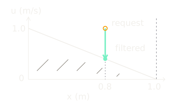
At $x=0.8$ m, margin is $0.2$ m, so forward velocity must be at most $0.4$ m/s. Given nominal command $u_{\rm nom}=1$ m/s and input bounds $-0.5\leq u\leq1$ m/s, solve

\min_u\ \tfrac12(u-u_{\rm nom})^2\quad\text{subject to}\quad -0.5\leq u\leq1,\quad u\leq0.4.

This scalar quadratic program is projection onto the interval $[-0.5,0.4]$ , so $u^*=0.4$ m/s. The diagram plots position horizontally and commanded forward velocity vertically. The sloping line is the barrier upper bound; lower commands are admissible within the input limits. At the same position, the vertical correction moves the nominal dot down to that line. This is a command-space picture, not a physical ramp or a predicted trajectory.

If the boundary command is recomputed continuously, $\dot h=-2h$ gives $h(t)=0.2e^{-2t}$ , which stays positive at every finite time. The controller approaches the modelled wall asymptotically. That calculation requires continuous state-dependent feedback, not a single held velocity.

What do sampling and inertia change?

Hold $u=0.4$ m/s from $x=0.8$ m for $\Delta t=0.1$ s. The next position is $0.84$ m, still allowed. Hold it for one second and the next position is $1.2$ m; the robot crosses the boundary after $0.5$ s. The initially valid derivative constraint did not remain valid throughout the hold. For this particular integrator, enforcing the boundary velocity each sample gives $h_{k+1}=(1-\gamma\Delta t)h_k$ , so $\gamma\Delta t\leq1$ is sufficient for nonnegative margin over the held interval. This special result is not a general sampled-data CBF theorem.

If the actual input is acceleration, state must include velocity: $\dot x=v$ , $\dot v=u$ . Then $\dot h=-v$ contains no $u$ ; the first derivative cannot constrain the acceleration command. A braking-aware safe set or a higher-order barrier is needed. A point only $0.2$ m from the wall at $1$ m/s cannot stop under a $1$ m/s² braking bound: its ideal stopping distance is $v^2/(2a)=0.5$ m. Including the measured position alone would admit a state from which avoidance is already impossible under that model.

What should happen when no command satisfies it?

With known drift $d$ , let $\dot x=u+d$ . The barrier bound becomes $u\leq2(1-x)-d$ . At the wall and $d=0.6$ m/s, it requires $u\leq-0.6$ m/s. The actuator only permits down to $-0.5$ m/s, so the feasible interval is empty. A solver must report that condition; a clipped command cannot restore the missing guarantee.

Barrier filtering can preserve a nominal policy locally while enforcing explicit model constraints. Its costs are state estimation, a suitable barrier, a feasible solve and real-time enforcement. Multiple individually feasible inequalities can conflict when combined. Slack on a safety inequality changes the claim, even if it improves solver availability. MPC is useful when future maneuver choices matter; a local barrier can stall without choosing a route around an obstacle. Discrete shielding uses a related intervention idea with different state and action assumptions. None replaces accurate models or complete hazard analysis.

Code

This offline scalar filter checks feasibility before projecting. It exposes a long sample hold and an actuator-limited failure rather than silently clipping either one away.

1from math import exp, isclose, isfinite2
3def filter_velocity(x: float, nominal: float, drift: float = 0.0,4                    gamma: float = 2.0) -> float | None:5    if not all(isfinite(v) for v in (x, nominal, drift, gamma)) or gamma <= 0:6        raise ValueError("finite values and positive gamma required")7    if x > 1.0:8        raise ValueError("initial state outside declared safe set")9    lower, upper = -0.5, min(1.0, gamma*(1.0-x)-drift)10    if upper < lower:11        return None12    return max(lower, min(upper, nominal))13
14x = 0.815u = filter_velocity(x, 1.0)16assert u is not None and isclose(u, 0.4)17assert filter_velocity(1.0, 1.0, drift=0.6) is None18assert filter_velocity(0.8, -0.2) == -0.219print(f"filtered velocity={u:.3f} m/s")20for dt in (0.1, 1.0):21    next_x = x+dt*u22    print(f"held {dt:.1f} s: x={next_x:.3f} m; inside={next_x <= 1.0}")23continuous_margin = (1-x)*exp(-2.0)24assert continuous_margin > 025print("drift at boundary: infeasible" if filter_velocity(1.0, 1.0, 0.6) is None26      else "feasible")

Output: filtered velocity=0.400 m/s, held 0.1 s: x=0.840 m; inside=True, held 1.0 s: x=1.200 m; inside=False, and drift at boundary: infeasible.

Watch Out For

A feasible optimizer result is called a physical guarantee

The mathematical constraint passes while stale sensing, unmodelled delay or limited braking carries the robot across the boundary. Match the input model to the actual interface, include relevant state such as velocity, and account for estimation error, disturbance bounds and sample holds in the argument. A residual checked once is evidence only at that evaluation.

Safety slack hides an empty feasible set

The controller reports a solution by relaxing the barrier inequality, then continues to claim invariance. Log constraint violations and infeasibility distinctly, keep actuator bounds inside the solve and define an evaluated response for the platform. Relaxing an objective can preserve a hard constraint; relaxing the hard constraint itself changes the promised property.

The Quick Version

A CBF constrains the margin's rate of change so a suitable feasible continuous controller keeps its model inside an allowed set.
At 0.2 m from the example wall, the constraint limits forward velocity to 0.4 m/s.
Sampling, inertia, disturbance and actuator bounds can invalidate a position-only continuous-feedback argument.
An empty feasible set must be reported; clipping or adding safety slack does not preserve the original guarantee.