Model Predictive Control for Robots

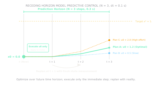
Model Predictive Control (MPC) optimizes robot commands across a future time horizon using a dynamic model, executes only the immediate first step, and replans at the next cycle with updated state feedback to handle constraints gracefully.

Model Predictive Control optimizes trajectories across a receding horizon, executing only the first action before replanning

Why Does This Exist?

Standard PID feedback control is purely reactive: it looks at present error $e(t)$ and past accumulated error to calculate motor torque. It cannot anticipate an upcoming sharp bend in a path, cannot look ahead to decelerate before hitting a hard joint limit, and cannot enforce complex inequality constraints (like maximum torque or obstacle boundaries).

Global motion planners (like A* or RRT) solve for long collision-free paths, but take hundreds of milliseconds to compute and assume a static world: if a human steps in front of the robot, the global planner stalls.

Model Predictive Control (MPC), also called receding horizon control, fills the vital middle tier between high-level global planning and low-level joint reflexes. By using a predictive mathematical model of robot physics over a short future window (such as $0.5$ to $2.0\text{ seconds}$ ), MPC optimizes candidate control sequences subject to hard physical constraints, executes only the first commanded step, and replans continuously with fresh sensor feedback.

Basics first: the low-level PID loops that track MPC setpoints live in robot-feedback-control. Global path planning across configuration space lives in robot-motion-planning. Learning action-conditioned predictive dynamics from data lives in robot-world-models.

Think of It Like This

Sprinting through a crowded train station while looking five paces ahead

Imagine rushing through a crowded train concourse to catch your departure. You do not stare straight down at your toes (purely reactive PID), nor do you freeze to calculate a rigid, fixed route across the entire building (global planning).

Instead, you focus your gaze five paces ahead (the prediction horizon). As you run, you predict where walking passengers will be in two seconds, steer smoothly around them, and avoid brushing against luggage carts (constraint handling).

Crucially, you only execute your very next stride. As your foot hits the ground, you shift your gaze forward another five paces and adjust your heading based on what actually moved.

Where it stops: human runners have vast situational awareness and peripheral vision. Robot MPC must solve a numerical mathematical optimization problem (such as a quadratic program) within strict real-time deadlines (e.g. every $10\text{ to }20\text{ milliseconds}$ ). If the solver fails to converge before the deadline, the robot has no command to send to its motors.

How It Actually Works

The receding horizon optimization problem

At discrete time $t$ , given current measured state $\mathbf{x}_t$ , MPC solves a constrained finite-horizon optimal control problem over a prediction horizon of $N$ steps:

\min_{\mathbf{u}_0, \mathbf{u}_1, \dots, \mathbf{u}_{N-1}} \sum_{k=0}^{N-1} \left( \|\mathbf{x}_k - \mathbf{x}^*\|_{\mathbf{Q}}^2 + \|\mathbf{u}_k\|_{\mathbf{R}}^2 \right) + \|\mathbf{x}_N - \mathbf{x}^*\|_{\mathbf{Q}_f}^2

subject to:

Dynamic model: $\mathbf{x}_{k+1} = f(\mathbf{x}_k, \mathbf{u}_k)$ with $\mathbf{x}_0 = \mathbf{x}_t$ .
State constraints: $\mathbf{x}_{\min} \le \mathbf{x}_k \le \mathbf{x}_{\max}$ (e.g. maximum velocity, position boundaries).
Actuator constraints: $\mathbf{u}_{\min} \le \mathbf{u}_k \le \mathbf{u}_{\max}$ (e.g. motor torque limits, acceleration bounds).

where $\mathbf{Q}$ penalizes state tracking errors, $\mathbf{R}$ penalizes control effort, and $\mathbf{Q}_f$ is the terminal cost.

The receding horizon loop

Measure current state $\mathbf{x}_t$ from robot state estimation.
Solve the optimization problem over horizon $[t, t+N]$ to obtain optimal sequence $\mathbf{U}^* = [\mathbf{u}_0^*, \mathbf{u}_1^*, \dots, \mathbf{u}_{N-1}^*]$ .
Apply only the first control action $\mathbf{u}_0^*$ to the robot motor controllers.
Discard the remaining planned actions $[\mathbf{u}_1^*, \dots, \mathbf{u}_{N-1}^*]$ .
Advance the clock to $t+1$ , obtain fresh sensor feedback, and repeat the optimization.

Because the optimization repeats every cycle with real-world state feedback, MPC continuously corrects for model inaccuracies, wheel slip, and unexpected disturbances.

Worked example: 1D cart regulation over a 3-step horizon

Consider a 1D robotic delivery cart tracking a target position $x^* = 1.0\text{ m}$ .

Discrete state dynamics: $x_{k+1} = x_k + v_k \Delta t$ , $v_{k+1} = v_k + u_k \Delta t$ , with $\Delta t = 0.1\text{ s}$ .
Initial state at $t$ : position $x_0 = 0.0\text{ m}$ , velocity $v_0 = 0.0\text{ m/s}$ .
Horizon length: $N = 3$ steps ( $0.3\text{ seconds}$ ).
Actuator constraint: acceleration $|u_k| \le 2.0\text{ m/s}^2$ .
Velocity constraint: $0.0 \le v_k \le 1.0\text{ m/s}$ .
Cost function weights: $Q = 1.0$ (tracking error), $Q_v = 0.5$ (velocity damping), $R = 0.1$ (control effort).

Evaluate candidate control sequence $\mathbf{U} = [1.2, 1.2, 0.0]\text{ m/s}^2$ :

Step $k=0 \to 1$ ( $u_0 = 1.2\text{ m/s}^2$ ): $x_1 = 0.0 + 0.0 \cdot 0.1 = 0.000\text{ m}, \quad v_1 = 0.0 + 1.2 \cdot 0.1 = 0.120\text{ m/s}$ $J_1 = (0.0 - 1.0)^2 + 0.5 \cdot (0.12)^2 + 0.1 \cdot (1.2)^2 = 1.000 + 0.0072 + 0.144 = 1.1512$
Step $k=1 \to 2$ ( $u_1 = 1.2\text{ m/s}^2$ ): $x_2 = 0.000 + 0.12 \cdot 0.1 = 0.012\text{ m}, \quad v_2 = 0.12 + 1.2 \cdot 0.1 = 0.240\text{ m/s}$ $J_2 = (0.012 - 1.0)^2 + 0.5 \cdot (0.24)^2 + 0.1 \cdot (1.2)^2 = 0.9761 + 0.0288 + 0.144 = 1.1489$
Step $k=2 \to 3$ ( $u_2 = 0.0\text{ m/s}^2$ ): $x_3 = 0.012 + 0.24 \cdot 0.1 = 0.036\text{ m}, \quad v_3 = 0.24 + 0.0 \cdot 0.1 = 0.240\text{ m/s}$ $J_3 = (0.036 - 1.0)^2 + 0.5 \cdot (0.24)^2 + 0.1 \cdot (0.0)^2 = 0.9293 + 0.0288 + 0.0 = 0.9581$

Total horizon cost:

J_{\text{total}} = 1.1512 + 1.1489 + 0.9581 = 3.2582

All constraints are satisfied ( $v_k \le 1.0\text{ m/s}$ , $u_k \le 2.0\text{ m/s}^2$ ). The controller executes only the immediate action $u_0 = 1.2\text{ m/s}^2$ , commands the motor drive, and re-evaluates the optimization at $t = 0.1\text{ s}$ from the newly measured position and velocity.

Code

This Python snippet defines a discrete MPC forward simulator, computes state rollouts, evaluates cost functions, and verifies the receding horizon first-step selection.

1def evaluate_mpc_candidate(2    u_seq: list[float],3    x_init: float = 0.0,4    v_init: float = 0.0,5    x_target: float = 1.0,6    dt: float = 0.1,7) -> tuple[float, float, float]:8    """Simulate candidate control sequence over horizon and return (cost, final_x, final_v)."""9    x: float = x_init10    v: float = v_init11    total_cost: float = 0.012
13    for u in u_seq:14        x_next: float = x + v * dt15        v_next: float = v + u * dt16        # Cost: tracking error + velocity penalty + control effort17        stage_cost: float = (x_next - x_target) ** 2 + 0.5 * (v_next ** 2) + 0.1 * (u ** 2)18        total_cost += stage_cost19        x, v = x_next, v_next20
21    return round(total_cost, 4), round(x, 4), round(v, 4)22
23
24cost, x_end, v_end = evaluate_mpc_candidate(u_seq=[1.2, 1.2, 0.0])25print(cost)   # -> 3.258226print(x_end)  # -> 0.03627print(v_end)  # -> 0.24

Watch Out For

Optimization solver exceeding real-time loop deadlines

If your robot's control loop runs at $50\text{ Hz}$ ( $20\text{ ms}$ period), an MPC solver (such as a nonlinear interior-point optimizer) must guarantee completion in well under $15\text{ ms}$ . If the optimizer gets stuck resolving non-convex obstacles, it misses its compute deadline.

The symptom is the robot stuttering, hesitating, or executing outdated commands while the control loop stalls. Fix it by using warm-starting (seeding the solver with the shifted solution from the previous cycle), setting strict maximum iteration caps, or using high-speed convex quadratic programming (OSQP, qpOASES).

Model mismatch inducing high-frequency chatter

If the internal predictive model assumes an idealized frictionless surface while the real robot operates on thick carpet, the predicted state trajectory diverges from physical reality within two steps.

The symptom is aggressive command chattering: at step $t$ the solver commands large positive torque expecting rapid motion, but at $t+1$ discovers the robot moved only half as far, causing it to command erratic corrections. Fix it by adding state-dependent disturbance estimators or learning data-driven robot world models that predict physical dynamics under complex contacts.

The Quick Version

Model Predictive Control optimizes control sequences across a finite future time horizon using a dynamic system model.
At each cycle, MPC solves a constrained optimization problem, executes only the first action ( $u_0$ ), and replans with fresh feedback.
For a 1D cart tracking $x^* = 1.0\text{ m}$ over a 3-step horizon ( $\Delta t = 0.1\text{ s}$ ), candidate sequence $[1.2, 1.2, 0.0]\text{ m/s}^2$ yields a cost of $3.2582$ .
MPC inherently respects physical inequality constraints, such as motor torque limits, maximum velocity envelopes, and obstacle clearance margins.
Real-time feasibility requires fast convex quadratic solvers and warm-starting to ensure the optimizer consistently finishes within its strict loop deadline.