Robot Observability: What Sensors Can Reveal

Why Does This Exist?

A range sensor reports 1.2 m. Is the robot at 1.0 m with a 0.2 m sensor offset, or at 0.8 m with a 0.4 m offset? Observability asks whether measurements over time can distinguish different initial states under a declared model. A filter cannot recover missing information merely by running longer.

A state is the set of quantities being estimated. A measurement is an observation predicted from that state. State estimation explains how to combine noisy evidence; this page asks whether that evidence separates the unknowns at all. System identification asks a related question about unknown model parameters. Here the motion law is known and a constant sensor bias is included in the state.

Think of It Like This

How It Actually Works

What does measurement history add?

For a discrete linear, time-invariant model, write

$s_{k+1}=As_k+Bu_k,\qquad z_k=Hs_k.$

Here $s_k$ is an $n$-component state at sample $k$, $u_k$ a known input, $z_k$ the measurement, and $A,B,H$ the transition, input and measurement matrices. Subtracting the known input contribution from the output history leaves a linear map of the initial state. Its first $n$ blocks form

$\mathcal O=\begin{bmatrix}H\\HA\\\vdots\\HA^{n-1}\end{bmatrix}.$

Full column rank $n$ means the initial state is uniquely recoverable in the ideal noiseless model. A nonzero vector $d$ satisfying $\mathcal O d=0$ is an invisible state difference. This construction and criterion follow MIT's observability notes, section 24.3. Rank concerns distinguishability, not measurement accuracy.

Work a position-and-bias ambiguity

Use a fixed corridor axis, positive toward increasing position. Let $s=[p,b]^T$, where position $p$ and constant additive sensor bias $b$ are in metres; $T$ means transpose. A stipulated sensor measures $z=p+b$. Assume exact known travel $u$ in metres, no process noise and no bias drift:

$A=\begin{bmatrix}1&0\\0&1\end{bmatrix},\quad B=\begin{bmatrix}1\\0\end{bmatrix},\quad H=\begin{bmatrix}1&1\end{bmatrix}.$

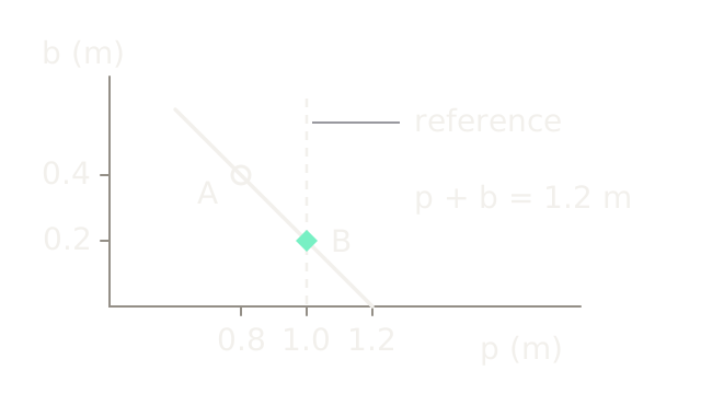
Candidate A is $(p,b)=(0.8,0.4)$ m; candidate B is $(1.0,0.2)$ m. Both give $z_0=1.2$ m. Move by $u=0.2$ m. Their next states are $(1.0,0.4)$ and $(1.2,0.2)$ m; both give $z_1=1.4$ m. Subtracting known travel gives $z_1-u=1.2$ m again.

Thus $\mathcal O=[[1,1],[1,1]]$ has rank one. The difference between candidates, $(0.2,-0.2)$ m, lies in its null space: increasing position and decreasing bias equally leaves every output unchanged. Any sequence of known additive travel preserves this ambiguity. Motion alone doesn't help this particular model.

Add one independently calibrated position observation $r=p=1.0$ m at the initial time. The combined equations are $p+b=1.2$ and $p=1.0$, so $b=0.2$ m. Their matrix $[[1,1],[1,0]]$ has determinant $-1$ and rank two. The diagram is state space, not a floor map: horizontal position and vertical bias both use 300 drawing units per metre, with the position axis cropped to start at 0.4 m. The descending line contains equivalent states. The dashed vertical reference selects the mint diamond at candidate B. It depicts noiseless equations; noisy readings would give regions rather than an exact intersection.

Why can one position sensor reveal velocity?

Change the model to $s=[p,v]^T$, with velocity $v$ in m/s and sampling interval $h>0$ seconds. Constant velocity gives $A=[[1,h],[0,1]]$ and $H=[1,0]$. Now $HA=[1,h]$, so the two-row determinant is $h$. Measurements at distinct times distinguish initial position and velocity: $v=(z_1-z_0)/h$ in the noiseless case.

Small $h$ still gives full rank, but differencing independent position noise of variance $\sigma^2$ produces velocity-error variance $2\sigma^2/h^2$. This follows by adding the two independent error variances before dividing by $h^2$. Faster paired readings can therefore give a noisier two-sample velocity estimate. A longer history can improve estimation under the correct model, while acceleration invalidates constant velocity over a long interval.

For practical design, scale states into meaningful reference units before interpreting singular values. Metres and m/s are different coordinates; a raw numerical condition number changes when units change. Weight output errors by sensor noise, inspect weak directions, and evaluate the intended motion and available observations together. Add a reference or alter sensor geometry when an ambiguity matters; adding a sensor increases calibration and timing work.

Robot models are often nonlinear and depend on trajectory. The linear rank test above is exact for the stated linear model, not a global observability proof for a camera-IMU system. An arbitrary SLAM origin is a reference choice, while an unconstrained physical bias can affect predictions. Keep those two reasons for a free direction separate. Use the existing partial-observability lesson for policy decisions under hidden state; a longer policy history doesn't automatically identify an unobservable physical quantity.

Code

This standalone Python constructs indistinguishable histories and then resolves the initial state with the independent reference. It also checks the velocity-noise amplification just derived.

1from math import isclose, sqrt2
3
4def history(position: float, bias: float, travel: list[float]) -> list[float]:5    readings = [position + bias]6    for step in travel:7        position += step8        readings.append(position + bias)9    return readings10
11
12a = history(0.8, 0.4, [0.2, -0.1, 0.3])13b = history(1.0, 0.2, [0.2, -0.1, 0.3])14assert all(isclose(x, y) for x, y in zip(a, b))15reference = 1.016bias = a[0] - reference17assert isclose(bias, 0.2)18print("same readings:", [round(z, 2) for z in a])19print(f"reference resolves p={reference:.1f} m, b={bias:.1f} m")20for h in (0.1, 1.0):21    sigma_v = sqrt(2) * 0.01 / h22    print(f"h={h:.1f} s: velocity noise sigma={sigma_v:.4f} m/s")

Output readings are [1.2, 1.4, 1.3, 1.6]. The reference resolves p=1.0 m, b=0.2 m; velocity noise standard deviations are 0.1414 and 0.0141 m/s respectively. These are synthetic model checks, not sensor specifications.

Watch Out For

The Quick Version

• Observability concerns whether measurement history distinguishes states under a particular dynamics model.
• Repeated measurements of position plus constant bias cannot separate those two quantities in the worked additive-motion model.
• An independent position reference resolves the example as position 1.0 m and bias 0.2 m.
• Full rank establishes ideal distinguishability; noise conditioning determines how usable that distinction is.
• A local linear test does not establish global observability of a nonlinear robot.

What to Read Next

• Robot State Estimation and Sensor Fusion
• Robot Inertial Navigation
• Robot System Identification: Learning the Physics
• Partial Observability