Robot System Identification: Learning the Physics
A robot's model needs numbers such as inertia and friction. Carefully chosen motions reveal those numbers; repeating an uninformative motion cannot.
Why Does This Exist?
A simulator contains an inertia value, but where did that value come from? A CAD estimate may omit a tool, a gearbox or a newly attached load. System identification estimates a system's model from measured inputs and responses. For a structured mechanical model, that can mean fitting inertia, friction or actuator parameters.
A state describes the current condition, such as joint position and velocity. A parameter describes the model, such as the inertia relating torque to acceleration. State estimation tracks changing state; identification asks which model parameters explain its changes. Some methods estimate both, but the questions remain distinct.
This lesson starts from robot dynamics with a known equation form. It shows why collecting varied data can matter more than collecting many repeated samples. Learning an unrestricted visual world model is a broader modelling problem, covered in world models.
Think of It Like This
Testing a loaded trolley on a level floor
Push a trolley while it rolls steadily and you mainly learn how much force balances its resistance. Push it so its speed changes and you also learn how hard it is to accelerate. If every trial repeats the same steady speed, a heavy freely rolling trolley and a lighter one can remain indistinguishable in mass from that experiment.
Applied push is input effort, changing motion is measured response, and the unknown load and resistance are model parameters. The analogy stops at its resistance law: real wheels can have static, rolling and speed-dependent friction. Our calculation uses a declared linear viscous term to make identifiability visible.
How It Actually Works
State a model the measurements can test
Use a synthetic horizontal rotary joint with no gravity torque or contact. Let be angular velocity in rad/s, angular acceleration in rad/s², and delivered joint torque in N m. Assume constant inertia in kg m² and linear viscous friction coefficient in N m s/rad:
The resisting friction torque is , so appears on the required-effort side. We assume calibrated, synchronized torque and motion values and omit motor dynamics, static friction, backlash and temperature drift. These are modelling assumptions, not properties guaranteed by a real joint.
For observation , write the row and parameter vector . Stack rows into data matrix and torques into vector . Then . The superscript means transpose. Least squares chooses minimizing , the sum of squared torque residuals. MIT's system-identification chapter develops structured mechanical parameter fitting and experiment design.
Which observations separate inertia from friction?
Take these independently stipulated, noiseless snapshots:
| Snapshot | Acceleration (rad/s²) | Velocity (rad/s) | Torque (N m) |
|---|---|---|---|
| Speeding up | 1 | 1 | 0.7 |
| Slowing down | -1 | 1 | -0.3 |
| Reverse steady motion | 0 | -1 | -0.2 |
The first two equations are and . Adding gives , so N m s/rad. Subtracting gives , so kg m². The third row checks N m. The coefficient of inertia changes sign between the first two observations while the coefficient of friction stays fixed; that lets us distinguish their effects.
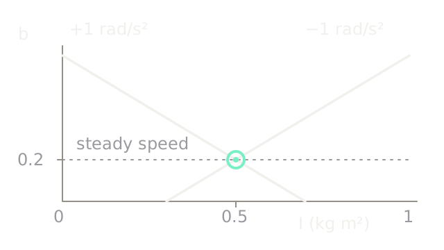
Each solid line in the diagram is a set of parameter pairs that explains one observation. One says ; the other says . They meet at the mint ring, . The horizontal axis is inertia; the vertical axis is viscous coefficient in N m s/rad. The lines describe possible models, not a joint's physical path through space.
For a held-out snapshot rad/s² and rad/s, the fitted model predicts N m. This is a synthetic consistency check, not experimental evidence that the model describes hardware.
Why doesn't more steady-speed data solve it?
At steady speed, , so inertia disappears from the equation. A row with rad/s and N m identifies , but allows every positive . This is the dotted horizontal line in parameter space. Repeating the row a thousand times can reduce some noise in the friction estimate; it supplies no inertia information. Setting in every row would also fail: then only the combination is identifiable.
The algebraic requirement is full column rank of for the parameters being estimated. Here the two columns must be independent. Near dependence produces a poorly conditioned problem: small measurement errors can cause large parameter changes. Persistent excitation is the related requirement that an input and its resulting motions keep supplying independent information over time. A finite full-rank dataset illustrates the principle without proving every online estimator's excitation assumptions.
On multi-link robots, even varied data may identify only combinations called base parameters, rather than every link parameter separately. Also scale the columns before interpreting a raw condition number: acceleration and velocity have different units and magnitudes. QR or singular-value decomposition is preferable to explicitly forming and inverting normal equations in a numerical implementation.
How do you tell a useful fit from a convenient fit?
Keep validation motions separate from fitting motions, including the operating range that matters to the controller. A small torque residual on training data is not a test of long-horizon motion. Roll out the fitted dynamics with recorded input and initial condition, then compare position and velocity traces. One-step and rollout errors answer different questions; robot simulation adds numerical solver and integration choices that can also affect the comparison.
Inspect residuals against velocity, acceleration, configuration and time. A residual changing sign with speed may suggest a missing friction term; a systematic time shift may suggest misalignment. Neither pattern alone diagnoses a unique cause. Filtered encoder derivatives are particularly delicate: noise is amplified by differentiation, while filtering can shift phase. Delivered torque derived from current also depends on torque constants, transmission effects and calibration.
Ordinary least squares assumes a suitable noise model. Noise in the regressors creates an errors-in-variables problem; feedback can correlate inputs with disturbances. Integral formulations, instrumental variables or prediction-error methods may be needed. Positive inertia constraints prevent an obviously impossible fit but don't make an uninformative dataset informative.
Use structured identification when known physics and a modest parameter set explain the behavior of interest. Use a richer model when residual structure persists under good measurements and excitation. Collecting that richer data and validating the model costs more than replacing a scalar fit with a larger optimizer. Plan excitation within the robot's motion and effort constraints, rather than treating aggressive motion as a substitute for informative experiment design.
Code
The tiny two-parameter solver below exposes the rank check and the scalar arithmetic. It forms normal-equation sums for transparency; use a scaled QR/SVD solver for noisy, larger or ill-conditioned problems.
def fit_joint(rows: list[tuple[float, float, float]]) -> tuple[float, float]: aa = sum(a * a for a, w, torque in rows) ww = sum(w * w for a, w, torque in rows) aw = sum(a * w for a, w, torque in rows) ay = sum(a * torque for a, w, torque in rows) wy = sum(w * torque for a, w, torque in rows) determinant = aa * ww - aw * aw if aa == 0 or ww == 0 or determinant <= 1e-10 * aa * ww: raise ValueError("data do not separate inertia and friction") return ((ay * ww - wy * aw) / determinant, (wy * aa - ay * aw) / determinant)
observations = [(1.0, 1.0, 0.7), (-1.0, 1.0, -0.3), (0.0, -1.0, -0.2)]inertia, friction = fit_joint(observations)prediction = inertia * 2 + friction * (-0.5)assert abs(inertia - 0.5) < 1e-12assert abs(friction - 0.2) < 1e-12assert abs(prediction - 0.9) < 1e-12print(f"I={inertia:.3f}, b={friction:.3f}, held-out torque={prediction:.3f}")try: fit_joint([(0.0, 1.0, 0.2)] * 100)except ValueError as error: print(error)else: raise AssertionError("steady-speed data cannot identify inertia")Output: I=0.500, b=0.200, held-out torque=0.900 and
data do not separate inertia and friction. Rejecting this dataset is the useful
result, rather than silently returning one arbitrary inertia.
Watch Out For
Repeated easy motions leave one parameter unconstrained
The training residual is tiny, but fitted inertia changes wildly between runs. Inspect rank and singular values after sensible column scaling. Choose admissible motions that vary independent parameter effects, then validate on separate motions. More repetitions of the same rank-deficient experiment won't resolve the ambiguity.
Friction absorbs a timestamp or effort error
An estimate changes sharply when the logging rate or filter setting changes. Check acquisition timestamps, filtering delay and whether torque is delivered effort or a pre-limit command. An optimizer can reduce residual by distorting parameters; it cannot establish that the measurement pipeline is physically correct.
The Quick Version
- System identification estimates a model from applied inputs and measured responses.
- Independent parameter effects must appear in the data; steady-speed motion alone cannot identify inertia.
- A low training residual doesn't establish identifiable parameters or accurate rollouts.
- Calibration, synchronization, measurement noise and controller feedback affect the estimator's validity.
- Validate the fitted model on separate motions over the operating conditions the controller will use.