Robot Inertial Navigation

An accelerometer feels support and thrust, not position. A robot must track its orientation, remove gravity in the right frame and integrate carefully to turn those readings into motion.

An orientation error leaves a false horizontal acceleration after gravity compensation.

Why Does This Exist?

A stationary robot can appear to accelerate if its orientation estimate is slightly tilted. Integrating that apparent acceleration twice produces a moving position estimate even though the robot never left its bench. Inertial navigation propagates orientation, velocity and position from an inertial measurement unit, or IMU; it needs initial conditions and accumulates error.

An IMU typically provides angular-rate and accelerometer readings along three body axes. Angular rate describes how fast the body turns; acceleration changes velocity, and velocity changes position. The prerequisite is knowing how to rotate vectors between frames. This page explains the propagation step; state estimation explains how external evidence can correct it.

Think of It Like This

A spring scale in an elevator

A mass hanging from a spring stretches it while the elevator rests. It stretches more as the elevator accelerates upward, and loses its load in ideal free fall. Reading the stretch alone doesn't tell you the elevator's position or even its acceleration until you account for gravity and the scale's direction.

The spring's load maps to accelerometer specific force, its direction to the sensor axes, and the elevator's motion to the robot's motion. The analogy stops at rotation sensing: a spring scale supplies no gyroscope reading and cannot establish all three orientation axes.

How It Actually Works

What does the accelerometer actually measure?

Choose a local world frame W with z upward and gravity $g_W=(0,0,-9.81)$ m/s² for our teaching calculations. Let $R$ map body-frame B vectors into W. An ideal accelerometer reports specific force

f_B=R^T(a_W-g_W),\qquad a_W=Rf_B+g_W.

$a_W$ is translational acceleration of the sensor origin, $f_B$ is force per unit mass along its axes, and $R^T$ reverses the rotation. At rest with aligned frames, $a_W=0$ , so $f_B=(0,0,+9.81)$ m/s². Adding the downward gravity vector then recovers zero. In ideal free fall $f_B=0$ , so $a_W=g_W$ . The CMU inertial-navigation lecture develops this distinction. Some drivers publish an already gravity-compensated acceleration stream; applying this formula to that stream compensates twice.

Measured specific force $f_m$ also contains accelerometer bias $b_a$ and noise. Gyroscope measurement $\omega_m$ contains angular velocity, gyro bias $b_g$ and noise. A bias is a persistent offset, not fresh independent noise at each sample.

How does one propagation interval work?

Ignoring Earth rotation over a short local interval, assume corrected body angular rate is constant over sample interval $\Delta t$ . Update orientation with

R_{k+1}=R_k\exp([\omega_m-b_g]_\times\Delta t).

The brackets form the skew matrix satisfying $[u]_\times v=u\times v$ ; the exponential turns that incremental angle into a rotation matrix. Right multiplication corresponds to body-frame angular rate. For changing rates, compose successive increments in order rather than exponentiating one accumulated vector of angles.

Using a representative orientation during that interval, compute $a_W=R(f_m-b_a)+g_W$ . For acceleration assumed constant in W over the interval,

v_{k+1}=v_k+a_W\Delta t,\qquad p_{k+1}=p_k+v_k\Delta t+\tfrac12a_W\Delta t^2.

$v$ is velocity in m/s and $p$ is position in metres. The position equation uses the old velocity. A midpoint orientation is preferable when significant rotation occurs during a sample; coning, vibration, timing error and sensor saturation demand more than this constant-input model. Woodman's Cambridge report, Sections 6.1–6.2, explains the orientation-to-position error path. Its historical hardware results are not performance specifications for today's IMUs.

Worked example: gravity leaks sideways

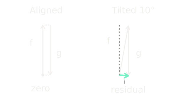
Keep the actual robot at rest and ignore sensor noise. Suppose the estimated orientation has a constant tilt $\epsilon$ about world y. It maps the measured upward vector to

\hat Rf_B=(9.81\sin\epsilon,0,9.81\cos\epsilon).

After adding gravity, the false acceleration is $(9.81\sin\epsilon,0,9.81(\cos\epsilon-1))$ . For the diagram's deliberately visible $10^\circ$ tilt, these components are $(1.703489,0,-0.149036)$ m/s². The left pair of opposite vectors cancels exactly; on the right, equal-length vectors miss because their directions disagree. The short closing arrow is the residual, not the robot's actual acceleration.

With a smaller $1^\circ$ constant error, horizontal acceleration is $0.171208$ m/s². Starting at zero horizontal velocity, ten seconds gives false speed $1.712081$ m/s and displacement $\tfrac12(0.171208)(10^2)=8.560405$ m. This is a deterministic sensitivity example, not a predicted sensor error distribution. Separately, a constant uncorrected accelerometer bias of $0.02$ m/s² alone gives $1$ m displacement error over the same interval.

IMUs supply motion information between external fixes and through brief visual outages, at the cost of bias calibration and fast error growth. They are unsuitable as indefinite standalone position references. Stationary accelerometer data can constrain tilt, but gravity supplies no heading reference and sustained linear acceleration can masquerade as tilt. Camera, wheel or other independent observations constrain different errors. A zero-velocity update is justified only when the sensor is actually stationary; a constant-speed platform is not stationary just because its accelerometer readings look steady.

Observability explains why adding a heading or bias variable to the estimator does not make it measurable. Check which state differences the available observations can distinguish before assigning confidence to them.

Code

This standalone propagation check uses a stationary IMU and a deliberately wrong fixed tilt. The closed-form result checks the integration loop rather than only printing its formula.

1from math import cos, isclose, radians, sin2
3def drift(tilt_deg: float, seconds: float, steps: int) -> tuple[float, float]:4    if seconds <= 0 or steps <= 0:5        raise ValueError("positive interval and step count required")6    dt = seconds / steps7    # R_y(tilt) applied to (0, 0, g), then add world gravity.8    angle, gravity = radians(tilt_deg), 9.819    acceleration = (gravity*sin(angle), gravity*(cos(angle)-1))10    p, v = [0.0, 0.0], [0.0, 0.0]11    for _ in range(steps):12        for j in range(2):13            p[j] += v[j]*dt + 0.5*acceleration[j]*dt*dt14            v[j] += acceleration[j]*dt15    assert isclose(p[0], 0.5*acceleration[0]*seconds**2, abs_tol=1e-10)16    return p[0], v[0]17
18assert drift(0.0, 10.0, 1000) == (0.0, 0.0)19x, speed = drift(1.0, 10.0, 1000)20print(f"false x={x:.6f} m; false vx={speed:.6f} m/s")21print(f"10-degree residual: {9.81*sin(radians(10)):.6f}, "22      f"{9.81*(cos(radians(10))-1):.6f} m/s^2")

Output: false x=8.560405 m; false vx=1.712081 m/s and 10-degree residual: 1.703489, -0.149036 m/s^2.

Watch Out For

Subtracting gravity before rotating sensor axes

A stationary sensor works upright but drifts when tilted. Gravity is a world-frame vector; compensate only after rotating the body reading, or rotate gravity into the body frame consistently. Check both an upright and a tilted stationary recording, including the driver's sign and compensation conventions.

A stationary calibration is treated as a universal zero

Bias removal succeeds on the bench but fails after temperature changes or during motion. A stationary reading includes gravity, so subtracting its entire vector as bias destroys the physical measurement model. Estimate bias with orientation accounted for, propagate bias uncertainty and use independent motion observations to correct drift.

The Quick Version

A raw accelerometer measures specific force; a stationary upward axis reads approximately positive g under this convention.
Rotate corrected specific force into the world frame, add gravity, then integrate using consistent timestamps.
A constant one-degree tilt error gives 8.560405 m of horizontal drift in the stated ten-second stationary example.
Inertial propagation bridges observations; it does not establish absolute position or eliminate the need for bias estimation.