Robot State Estimation and Sensor Fusion

Robots never directly observe their true physical state; they infer it by fusing noisy, asynchronous, and biased sensor streams through dynamic models. Sensor fusion combines fast, drifting odometry with slower, absolute corrections to bound uncertainty.

Sensor fusion combines an uncertain odometry prior with a landmark measurement, yielding a sharper posterior state estimate

Why Does This Exist?

If you ask a robot where it is, no single sensor can tell the truth. Wheel encoders measure wheel rotations with microsecond precision, but when the wheels slip on dusty concrete, the encoders claim the robot moved forward while it remained stationary. An inertial measurement unit (IMU) reports accelerations at $1000\text{ Hz}$ , but integrating raw accelerometer signals twice to compute position drifts into kilometers of error within seconds due to temperature bias. A camera or LiDAR can recognize landmarks accurately, but operates at only $20\text{ Hz}$ to $30\text{ Hz}$ and suffers from motion blur.

State estimation is the mathematical machinery that turns these flawed, asynchronous, and noisy observations into an optimal, continuous estimate of physical state $\mathbf{x}_t$ (such as 3D position, velocity, orientation, and sensor bias).

The core insight is Bayesian sensor fusion: instead of trusting any single instrument, the robot maintains a probability distribution over its state. It uses high-frequency motion models to predict state evolution, then uses incoming measurements to pull the estimate toward reality while shrinking its uncertainty.

Basics first: the general mathematical derivation of optimal linear filtering lives in kalman-filters. Building dense 3D geometry from camera depth lives in robot-perception-geometry. Using state estimates to track paths lives in robot-feedback-control.

Think of It Like This

Navigating a sailboat in dense fog with a knotmeter and a lighthouse

Imagine helming a sailboat through a thick fog bank toward a harbor entrance. You have two sources of information:

A water knotmeter and compass on your helm that measure boat speed through the water and heading continuously.
An occasional brief flash from a distant coastal lighthouse through the fog.

If you rely only on the knotmeter, ocean cross-currents and rudder drift slowly push you off course. Every minute without an external reference expands your circle of uncertainty on the chart.

Suddenly, the lighthouse flashes through the fog. That single bearing measurement has some optical uncertainty, but it provides an absolute anchor to the physical earth. You combine your running dead-reckoning estimate with the lighthouse flash: you adjust your helm position toward the lighthouse line of sight, and your circle of uncertainty snaps back down to a tight, confident radius.

Where it stops: a human navigator uses judgment and sea charts. A robotic state estimator executes rigorous matrix algebra at hundreds of Hertz, simultaneously tracking physical position while continuously estimating the sensor's own internal drift and bias parameters.

How It Actually Works

The predict-update cycle

State estimation models physical reality as a discrete stochastic state-space system:

State vector $\mathbf{x}_t$ : The true physical state (e.g. $[x, y, \theta, v_x, v_y, \omega, b_{\text{acc}}, b_{\text{gyro}}]^T$ ).
Process model: $\mathbf{x}_t = \mathbf{F} \mathbf{x}_{t-1} + \mathbf{B} \mathbf{u}_t + \mathbf{w}_t$ , where $\mathbf{w}_t \sim \mathcal{N}(\mathbf{0}, \mathbf{Q})$ is process noise with covariance $\mathbf{Q}$ .
Measurement model: $\mathbf{z}_t = \mathbf{H} \mathbf{x}_t + \mathbf{v}_t$ , where $\mathbf{v}_t \sim \mathcal{N}(\mathbf{0}, \mathbf{R})$ is measurement noise with covariance $\mathbf{R}$ .

The filter alternates between two steps:

Predict (Time Propagation): High-frequency IMU and wheel odometry propagate the state forward in time. Because process noise $\mathbf{Q}$ is added at every step, the covariance $\mathbf{P}$ (uncertainty) grows:
$\hat{\mathbf{x}}_t^- = \mathbf{F} \hat{\mathbf{x}}_{t-1} + \mathbf{B} \mathbf{u}_t$ $\mathbf{P}_t^- = \mathbf{F} \mathbf{P}_{t-1} \mathbf{F}^T + \mathbf{Q}$
Update (Measurement Correction): When an exteroceptive measurement $\mathbf{z}_t$ arrives (e.g. a camera landmark or LiDAR scan), the filter computes the Kalman Gain $\mathbf{K}_t$ , which balances prior uncertainty $\mathbf{P}_t^-$ against measurement noise $\mathbf{R}$ :
$\mathbf{K}_t = \mathbf{P}_t^- \mathbf{H}^T (\mathbf{H} \mathbf{P}_t^- \mathbf{H}^T + \mathbf{R})^{-1}$
The state is corrected using the innovation residual $(\mathbf{z}_t - \mathbf{H} \hat{\mathbf{x}}_t^-)$ :
$\hat{\mathbf{x}}_t = \hat{\mathbf{x}}_t^- + \mathbf{K}_t (\mathbf{z}_t - \mathbf{H} \hat{\mathbf{x}}_t^-)$
The uncertainty shrinks:
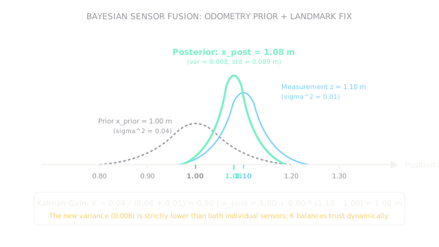
$\mathbf{P}_t = (\mathbf{I} - \mathbf{K}_t \mathbf{H}) \mathbf{P}_t^-$

Worked example: 1D sensor fusion of odometry and external fix

Consider a mobile delivery base moving along a 1D corridor:

Prior estimate from wheel odometry: $\hat{x}^- = 1.00\text{ m}$ .
Prior variance: $\sigma_-^2 = 0.04\text{ m}^2$ (standard deviation $\sigma_- = 0.20\text{ m}$ ).
External landmark measurement from LiDAR: $z = 1.10\text{ m}$ .
Measurement noise variance: $R = 0.01\text{ m}^2$ (standard deviation $\sigma_z = 0.10\text{ m}$ ).

Compute the Kalman gain $K$ :

K = \frac{\sigma_-^2}{\sigma_-^2 + R} = \frac{0.04}{0.04 + 0.01} = \frac{0.04}{0.05} = 0.80

Compute the corrected posterior state estimate $\hat{x}^+$ :

\hat{x}^+ = \hat{x}^- + K (z - \hat{x}^-) = 1.00 + 0.80 (1.10 - 1.00) = 1.00 + 0.80(0.10) = 1.08\text{ m}

Compute the updated posterior variance $\sigma_+^2$ :

\sigma_+^2 = (1 - K) \sigma_-^2 = (1 - 0.80) \times 0.04 = 0.20 \times 0.04 = 0.008\text{ m}^2

Compute the new standard deviation $\sigma_+$ :

\sigma_+ = \sqrt{0.008} \approx 0.0894\text{ m}

Because the external measurement is four times more precise than the prior ( $R = 0.01$ versus $\sigma_-^2 = 0.04$ ), the Kalman gain weights the measurement heavily ( $K = 0.80$ ). The resulting posterior estimate ( $1.08\text{ m}$ ) has an uncertainty ( $0.089\text{ m}$ ) that is strictly smaller than either the odometry prior ( $0.20\text{ m}$ ) or the raw measurement alone ( $0.10\text{ m}$ ).

Code

This Python snippet implements the 1D Kalman update equations, verifies the numerical result, and demonstrates how unmodeled wheel slip degrades state estimation.

1def kalman_update_1d(2    x_prior: float,3    var_prior: float,4    measurement: float,5    var_meas: float,6) -> tuple[float, float, float, float]:7    """Perform 1D scalar Bayesian update of state and variance."""8    k_gain: float = var_prior / (var_prior + var_meas)9    x_post: float = x_prior + k_gain * (measurement - x_prior)10    var_post: float = (1.0 - k_gain) * var_prior11    std_post: float = var_post ** 0.512    return round(k_gain, 3), round(x_post, 3), round(var_post, 4), round(std_post, 4)13
14
15k, x_fused, var_fused, std_fused = kalman_update_1d(16    x_prior=1.00,17    var_prior=0.04,18    measurement=1.10,19    var_meas=0.01,20)21
22print(k)          # -> 0.823print(x_fused)    # -> 1.0824print(var_fused)  # -> 0.00825print(std_fused)  # -> 0.0894

Watch Out For

Overconfident process noise tuning leading to filter divergence

If you tune the filter's process noise covariance $\mathbf{Q}$ too small, you are mathematically telling the estimator that the motion model is nearly perfect. Over time, the calculated covariance $\mathbf{P}$ shrinks toward zero.

Once $\mathbf{P}$ is infinitesimally small, the Kalman Gain $\mathbf{K}$ drops to zero: the filter stops listening to real incoming measurements. If the robot hits a slick patch of floor or collides with an obstacle, the filter stubbornly reports smooth motion along the planned path while the physical hardware sits stalled against a wall. Fix it by keeping $\mathbf{Q}$ realistically conservative and injecting noise during wheel slip.

Ignoring sensor timestamp latency and asynchronous arrival

In real robot middleware (such as ROS 2), sensor packets arrive over Ethernet or USB with variable delay: an IMU message from $1\text{ ms}$ ago might arrive after a camera frame captured $60\text{ ms}$ ago.

If an estimator naively applies measurement updates in the order packets arrive at the CPU, it updates current state with past observations, corrupting the covariance matrix and inducing severe ringing. Fix it by maintaining a fixed-lag buffer of historical states, rolling the filter state back to the measurement's timestamp, applying the update, and re-propagating forward.

The Quick Version

Robots infer internal and external physical state by fusing noisy, multi-rate, and drifting sensors through dynamic models.
The predict-update cycle propagates state forward with high-rate odometry and IMU, then corrects state and shrinks uncertainty with external fixes.
Kalman gain $K$ automatically weights the measurement relative to the prior: higher sensor precision yields a higher gain and larger state correction.
Fusing a prior at $1.00\text{ m}$ (variance $0.04$ ) with a landmark fix at $1.10\text{ m}$ (variance $0.01$ ) produces a posterior at $1.08\text{ m}$ with variance $0.008$ .
Estimators must explicitly estimate sensor biases (such as gyro drift) and manage asynchronous packet arrival times to avoid filter divergence.