Reinforcement Learning for Robot Control

Reinforcement learning trains robot control policies through trial-and-error interaction, discovering dynamic behaviors like quadruped locomotion and agile parkour. Rather than commanding raw motor voltages, modern RL policies output target setpoints to high-frequency PD controllers while optimizing shaped reward functions.

Reinforcement learning trains high-level policies at 50 Hz that command target setpoints to 1000 Hz joint PD controllers

Why Does This Exist?

Classical legged locomotion and dynamic robotics historically relied on analytical control models: Zero Moment Point (ZMP), inverted pendulum models, and whole-body quadratic programming. While these methods produce stable walking on flat laboratory floors, they struggle on rough gravel, slippery snow, and unstructured outdoor terrain where foot contact slippage cannot be predicted analytically.

Reinforcement Learning (RL) abandons hand-derived gait equations in favor of direct policy optimization: an agent interacts with a physics simulation across millions of simulated steps, receives scalar rewards for progressing forward without falling, and optimizes its neural network weights using policy gradient methods (such as Proximal Policy Optimization).

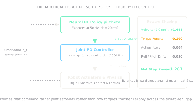
However, applying standard RL to physical robots fails if treated as an abstract game. If a neural network directly outputs raw motor voltages or currents at $50\text{ Hz}$ , high-frequency dynamics destabilize the actuators, causing severe joint vibration and motor burnout. Modern physical RL succeeds by embedding the learned policy inside a two-rate control hierarchy: the policy outputs target joint position offsets at $50\text{ Hz}$ , while dedicated low-level microcontrollers run proportional-derivative (PD) tracking loops at $1000\text{ Hz}$ .

Basics first: the physics simulators where millions of parallel RL steps run live in robot-simulation. The mathematical derivation of policy gradients lives in proximal-policy-optimization. Designing scalar rewards that prevent undesirable agent behavior lives in reward-shaping.

Think of It Like This

A jockey riding a galloping racehorse

Think of the division of labor between a jockey and a galloping thoroughbred horse running across uneven pasture.

The jockey does not command each leg muscle individually: they do not calculate knee flexion or hoof impact timing. The jockey sits in the saddle, assesses the overall direction, sets the pace, and nudges the reins every second (a $1\text{ Hz}$ to $2\text{ Hz}$ high-level policy).

The horse's spinal reflexes and cerebellum handle the high-speed biomechanics: adjusting muscle tension as hooves hit mud, stabilizing the ankle upon impact, and managing ground reaction forces at hundreds of Hertz.

Where it stops: a horse has millions of years of biological evolution and self-preservation instincts. A quadruped robot's policy has only the rewards you program into its loss function: if you reward forward speed without penalizing joint torque or impact vibration, the policy will discover gaits that slam steel feet into concrete until the motor gears fracture.

How It Actually Works

The Markov decision process for legged locomotion

Robot RL formulates continuous physical control as a Markov Decision Process (MDP) defined by $(\mathcal{S}, \mathcal{A}, \mathcal{P}, \mathcal{R}, \gamma)$ :

Observation Space $\mathbf{o}_t \in \mathbb{R}^{48}$ : Typically composed of:
- Base angular velocity $\boldsymbol{\omega}_b \in \mathbb{R}^3$ from IMU gyroscopes.
- Projected gravity vector $\mathbf{g}_b \in \mathbb{R}^3$ in the chassis frame.
- Commanded velocity target $\mathbf{v}^* = [v_x^*, v_y^*, \omega_z^*]^T$ .
- Joint positions $\mathbf{q} \in \mathbb{R}^{12}$ and velocities $\dot{\mathbf{q}} \in \mathbb{R}^{12}$ (for a 12-DoF quadruped).
- Previous action vector $\mathbf{a}_{t-1} \in \mathbb{R}^{12}$ .
Action Space $\mathbf{a}_t \in \mathbb{R}^{12}$ : Target joint position offsets $\Delta \mathbf{q}^*$ . The commanded joint setpoint is $\mathbf{q}_{\text{target}} = \mathbf{q}_{\text{default}} + \mathbf{a}_t$ .
Low-Level Motor Reflex: At each $1\text{ ms}$ interval ( $1000\text{ Hz}$ ), the actuator microcontroller computes torque: $\boldsymbol{\tau}_t = \mathbf{K}_p (\mathbf{q}_{\text{target}} - \mathbf{q}_t) - \mathbf{K}_d \dot{\mathbf{q}}_t$

Reward shaping for physical feasibility

If an agent is rewarded solely for forward speed ( $r_t = v_x$ ), it discovers unphysical, violent gaits that break real hardware. Robust robot RL employs multi-objective reward shaping that balances task accomplishment against energy consumption, smoothness, and structural survival:

r_t = r_{\text{vel}} + r_{\text{ang}} + r_{\text{torque}} + r_{\text{action\_rate}} + r_{\text{orientation}}

Tracking reward: $r_{\text{vel}} = w_v \exp\left(-\frac{\|\mathbf{v}_{xy} - \mathbf{v}^*\|^2}{\sigma_v^2}\right)$ , granting positive reward when linear velocity matches the target.
Torque penalty: $r_{\text{torque}} = -w_\tau \|\boldsymbol{\tau}\|^2$ , discouraging excessive motor heating.
Action smoothness penalty: $r_{\text{action\_rate}} = -w_a \|\mathbf{a}_t - \mathbf{a}_{t-1}\|^2$ , penalizing jerky control setpoints.
Base orientation penalty: $r_{\text{orientation}} = -w_o (\|\omega_{\text{roll}}\|^2 + \|\omega_{\text{pitch}}\|^2)$ , enforcing an upright chassis.

Worked example: calculating shaped reward for quadruped locomotion

Consider a 12-DoF quadruped tracking a forward velocity command $v^* = 1.0\text{ m/s}$ :

Measured forward velocity: $v_x = 0.90\text{ m/s}$ (velocity tracking error $= 0.10\text{ m/s}$ ).
Total motor torque norm: $\|\boldsymbol{\tau}\| = 10.0\text{ N}\cdot\text{m}$ .
Action change norm: $\|\mathbf{a}_t - \mathbf{a}_{t-1}\| = 0.20\text{ rad}$ .
Base angular roll and pitch rate: $\omega_{\text{roll}} = 0.05\text{ rad/s}, \omega_{\text{pitch}} = 0.05\text{ rad/s}$ .
Reward weights:
- $w_v = 1.5, \quad \sigma_v = 0.50\text{ m/s} \implies \sigma_v^2 = 0.25$
- $w_\tau = 0.001$
- $w_a = 0.10$
- $w_o = 0.50$

Compute each term:

Velocity Tracking Reward: $r_{\text{vel}} = 1.5 \exp\left(-\frac{(0.90 - 1.00)^2}{0.25}\right) = 1.5 \exp\left(-\frac{0.01}{0.25}\right) = 1.5 \exp(-0.04) \approx 1.5 \times 0.960789 = 1.4412$
Torque Effort Penalty: $r_{\text{torque}} = -0.001 \times (10.0)^2 = -0.001 \times 100.0 = -0.1000$
Action Smoothness Penalty: $r_{\text{action\_rate}} = -0.10 \times (0.20)^2 = -0.10 \times 0.04 = -0.0040$
Chassis Orientation Penalty: $r_{\text{orientation}} = -0.50 \times (0.05 + 0.05) = -0.50 \times 0.10 = -0.0500$

Summing the components yields the net step reward:

r_{\text{total}} = 1.4412 - 0.1000 - 0.0040 - 0.0500 = 1.2872

The positive velocity progress ( $+1.441$ ) comfortably outweighs the combined mechanical and orientation penalties ( $-0.154$ ), guiding the policy gradient to reinforce this smooth, efficient gait.

Code

This Python snippet simulates one environment step of a quadruped locomotion policy, computing motor PD torques and evaluating shaped reward terms.

1import math2import numpy as np3
4
5def compute_locomotion_reward(6    v_actual: float,7    v_target: float,8    torque_norm: float,9    action_diff_norm: float,10    roll_rate: float,11    pitch_rate: float,12) -> tuple[float, float, float, float, float]:13    """Compute individual shaped reward components and net scalar reward."""14    # Velocity tracking term15    r_vel: float = 1.5 * math.exp(-((v_actual - v_target) ** 2) / 0.25)16
17    # Penalties18    p_torque: float = -0.001 * (torque_norm ** 2)19    p_action: float = -0.10 * (action_diff_norm ** 2)20    p_rot: float = -0.50 * (abs(roll_rate) + abs(pitch_rate))21
22    r_net: float = r_vel + p_torque + p_action + p_rot23    return (24        round(r_vel, 4),25        round(p_torque, 4),26        round(p_action, 4),27        round(p_rot, 4),28        round(r_net, 4),29    )30
31
32r_v, p_t, p_a, p_r, r_tot = compute_locomotion_reward(33    v_actual=0.90,34    v_target=1.00,35    torque_norm=10.0,36    action_diff_norm=0.20,37    roll_rate=0.05,38    pitch_rate=0.05,39)40
41print(r_v)    # -> 1.441242print(p_t)    # -> -0.143print(p_a)    # -> -0.00444print(p_r)    # -> -0.0545print(r_tot)  # -> 1.2872

Watch Out For

Directly outputting raw motor torques from neural network layers

Allowing an RL policy to command raw motor torques directly bypasses the motor drive's low-level feedback stabilization. Because neural networks operating at $50\text{ Hz}$ cannot adjust torque between policy calls, any contact bounce during foot strike causes the foot to bounce uncontrollably.

The symptom is high-frequency joint vibrations, stripped gearbox teeth, and extreme policy instability during contact transitions. Fix it by commanding target joint positions to a high-rate ( $1000\text{ Hz}$ ) PD controller, which inherently provides mechanical stiffness and damping at impact.

Reward hacking through unconstrained contact frequencies

When designing reward terms for walking or climbing, policies frequently exploit flaws in penalty weights: if foot clearance is rewarded without penalizing ground impact force, quadrupeds learn to violently slap their front paws into the ground at high frequencies.

The symptom is the policy reporting massive training rewards while performing an unnatural, violent vibration that would shatter physical hardware. Fix it by monitoring curriculum metrics: inspect torque norms, ground reaction force spikes, and foot contact durations, tightening penalties whenever unnatural behaviors emerge.

The Quick Version

Reinforcement learning discovers dynamic locomotion and agile manipulation through trial-and-error simulation training.
Physical RL uses a two-rate architecture: the neural policy outputs joint position targets at $50\text{ Hz}$ , while microcontroller PD loops compute torques at $1000\text{ Hz}$ .
Multi-objective reward shaping balances task velocity tracking against penalties on torque, action rate of change, and chassis orientation drift.
For a $1.0\text{ m/s}$ locomotion target, an actual speed of $0.90\text{ m/s}$ with torque norm $10\text{ N}\cdot\text{m}$ yields a net step reward of $1.2872$ .
Commanding target joint setpoints rather than raw torques provides essential physical damping during ground impacts.