Deploying Robot Policies Across the Reality Gap

Bridging the sim-to-real gap requires more than domain randomization. It demands explicit sensor-action contracts, rate clamping, and latency-tolerant action queues that protect real actuators from unmodeled delays and erratic neural network predictions.

Why Does This Exist?

A policy trained to 99% task success in simulation or on clean teleoperation traces often shudders, stalls, or crashes violently within seconds of being loaded onto physical hardware.

The immediate temptation is to blame physics mismatches—assuming the friction coefficient was slightly wrong or the mass was underestimated. But on real hardware, the primary failure mode during policy deployment is almost always an unmodeled sensor-action contract violation:

Latency misalignment: In simulation, observation acquisition, policy evaluation, and action execution happen instantaneously in lockstep. On physical hardware, reading a depth camera takes $30\text{ ms}$ , neural network inference over a GPU takes $30\text{ ms}$ , and communication over a CAN or EtherCAT bus adds another $5\text{ ms}$ . If the robot executes an action computed from a $65\text{ ms}$ old state while traveling at speed, control commands lag behind reality, triggering severe phase lag and oscillatory instability.
Frequency and rate discontinuities: Low-level motor controllers run feedback loops at $500\text{ Hz}$ to $1000\text{ Hz}$ . Neural network policies, especially vision-based foundation models, can rarely execute faster than $10\text{ Hz}$ to $50\text{ Hz}$ . Directly streaming raw neural network outputs to physical motor drives creates jagged, high-frequency torque spikes that strip gearbox teeth and trigger thermal cutoffs.
Distribution shift and out-of-bounds exploration: In simulation, exploring an unnatural configuration costs nothing; the environment simply resets. On hardware, a single out-of-distribution observation can cause a neural policy to command a joint velocity that snaps a tendon or slams the end-effector into the tabletop.

Deploying a policy across the reality gap requires building an explicit hardware deployment wrapper: an architectural bridge that enforces safety clamps, smooths action trajectories, and buffers asynchronous inference pipelines so the physical robot operates continuously and safely.

Think of It Like This

Think of deploying a neural network policy onto a physical robot like putting an autonomous race car software trained in a video game behind the wheel of a real 500-horsepower sports car.

In the racing video game, input latency is zero, the road surface is an idealized mathematical plane, and turning the steering wheel instantly changes the vehicle heading. The virtual driver develops aggressive driving habits: snapping the virtual wheel $90^\circ$ in a single frame to initiate a turn.

When placed in a real sports car, steering violently in a fraction of a second would shear the steering column or spin the car out of control. Furthermore, hydraulic valves take time to open, tires compress, and the video feed from the windshield camera arrives with a 30-millisecond delay.

A deployment safety wrapper acts like the real car's Electronic Stability Control (ESC) and hydraulic power steering limiter. No matter how violently or erratically the sim-trained driver yanks the wheel, the ESC inspects the vehicle's actual tire slip, clamps the rate of steering angle change to what the mechanical chassis can tolerate, and interpolates commands smoothly over time.

Where the analogy stops: Automobile ESC operates primarily on vehicle slip angles and wheel braking. A robot deployment wrapper must handle multidimensional joint boundaries, Cartesian workspace bounding boxes, camera exposure mismatches, and asynchronous action queue management across multi-rate sensor buses.

How It Actually Works

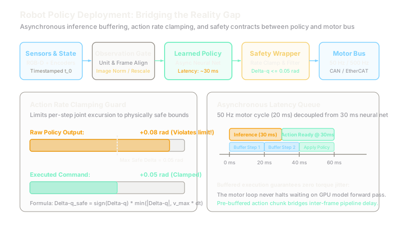
Deploying a learned policy onto real hardware requires structuring the execution runtime into three decoupled asynchronous tiers:

1[Sensors: 30-60 Hz] ──> [Observation Buffer] ──> [Async Policy GPU: 10-50 Hz]2                                                        │3                                                 (Action Chunk)4                                                        ▼5[Low-Level Motor Bus: 500 Hz] <── [Rate Clamping & Interpolation Queue]

1. The Sensor-Action Contract

Before passing physical observations into a neural policy, the deployment runtime must verify and enforce the sensor-action contract:

Coordinate conventions: If the policy was trained assuming optical frame conventions ( $Z$ -forward, $X$ -right, $Y$ -down), passing raw camera frames from a ROS optical driver without transform verification causes inverted actions.
Unit and normalization bounds: Learned policies expect observations normalized to $[\mu=0, \sigma=1]$ or $[-1, 1]$ . An unscaled millimeter reading passed into a model expecting meters produces instant saturation.
Latency compensation: If policy inference latency $\tau_{\text{inf}}$ is significant relative to the control period $\Delta t$ , the input to the policy must include the robot's current predicted state at the time the action will actually hit the motors ( $t + \tau_{\text{inf}}$ ), rather than the historical state captured when the camera shutter clicked ( $t$ ).

2. Action Rate Limiting

Learned policies can output discontinuous setpoints between successive cycles. To prevent hardware damage, the deployment wrapper applies an action rate clamp before passing setpoints to joint controllers.

Let $q_k$ be the current joint position, and $q_{k+1}^{\text{raw}}$ be the target position commanded by the policy for timestep $k+1$ . The time step is $\Delta t$ , and the maximum allowed joint angular velocity is $\dot{q}_{\max}$ .

The maximum allowable displacement per control step is:

\Delta q_{\max} = \dot{q}_{\max} \Delta t

The raw requested delta is:

\Delta q_{\text{raw}} = q_{k+1}^{\text{raw}} - q_k

The safe, clamped command $q_{k+1}^{\text{safe}}$ sent to the actuator bus is:

q_{k+1}^{\text{safe}} = q_k + \operatorname{sgn}(\Delta q_{\text{raw}}) \cdot \min\left(|\Delta q_{\text{raw}}|, \Delta q_{\max}\right)

If $|\Delta q_{\text{raw}}| > \Delta q_{\max}$ , the rate limiter flags a rate-clamping intervention. If consecutive interventions exceed a safety threshold, the system triggers a controlled stop.

3. Worked Example: Rate Clamping and Latency Queue

Consider a 6-DOF tabletop robot arm executing a policy at $\Delta t = 20\text{ ms}$ ( $50\text{ Hz}$ ).

Maximum safe elbow joint velocity: $\dot{q}_{\max} = 2.50\text{ rad/s}$ .
Maximum allowed joint step: $\Delta q_{\max} = 2.50 \times 0.020 = 0.050\text{ rad} \quad (\approx 2.86^\circ)$
Current elbow joint angle at step $k$ : $q_k = 0.820\text{ rad}$ .
Raw policy output setpoint: $q_{k+1}^{\text{raw}} = 0.900\text{ rad}$ .

Compute the raw requested displacement:

\Delta q_{\text{raw}} = 0.900 - 0.820 = +0.080\text{ rad}

Because $0.080\text{ rad} > 0.050\text{ rad}$ , the raw command exceeds the joint velocity threshold by $60\%$ . Directly commanding this setpoint would draw excessive current and trigger an over-torque fault.

The rate limiter clamps the step:

q_{k+1}^{\text{safe}} = 0.820 + 0.050 = 0.870\text{ rad}

The remaining $0.030\text{ rad}$ of desired travel is deferred to subsequent steps.

Now consider the timing budget:

Camera capture and preprocessing: $15\text{ ms}$ .
Neural network forward pass: $30\text{ ms}$ .
Total pipeline latency: $45\text{ ms}$ ( $2.25$ control cycles).

To prevent the low-level motor loop from starving during this $45\text{ ms}$ window, the deployment runtime uses action chunking with an asynchronous ring buffer. When the policy emits an action chunk of $H = 8$ steps ( $160\text{ ms}$ of planned motion), the high-frequency motor controller pops verified actions from the queue every $20\text{ ms}$ . When the next policy inference completes at $t = 45\text{ ms}$ , the buffer blends the new trajectory chunk smoothly into the active queue, eliminating motor stutter.

Code

The following Python script implements a production-grade deployment wrapper that validates observation freshness, clamps joint velocity excursions, and manages an asynchronous action buffer:

1from dataclasses import dataclass2import time3from typing import List, Optional, Tuple4
5
6@dataclass7class RobotState:8    timestamp: float9    joint_positions: List[float]10
11
12class HardwareDeploymentWrapper:13    """Wraps a learned policy for safe real-time physical deployment."""14
15    def __init__(16        self,17        num_joints: int,18        control_dt: float = 0.020,  # 50 Hz19        max_joint_vel: float = 2.50,  # rad/s20        max_observation_age: float = 0.100,  # 100 ms timeout21    ) -> None:22        self.num_joints = num_joints23        self.dt = control_dt24        self.max_delta_q = max_joint_vel * control_dt  # 0.050 rad25        self.max_obs_age = max_observation_age26        self.action_queue: List[List[float]] = []27        self.last_safe_command: Optional[List[float]] = None28
29    def validate_observation(self, state: RobotState, current_time: float) -> bool:30        """Reject stale observations caused by camera frame drops or bus delays."""31        age = current_time - state.timestamp32        if age > self.max_obs_age:33            return False34        return True35
36    def clamp_action_step(37        self, current_q: List[float], target_q: List[float]38    ) -> Tuple[List[float], bool]:39        """Clamps joint delta to maximum permissible step size."""40        clamped_cmd: List[float] = []41        was_clamped = False42
43        for q_curr, q_targ in zip(current_q, target_q):44            delta = q_targ - q_curr45            if abs(delta) > self.max_delta_q:46                clamped_delta = self.max_delta_q if delta > 0 else -self.max_delta_q47                clamped_cmd.append(q_curr + clamped_delta)48                was_clamped = True49            else:50                clamped_cmd.append(q_targ)51
52        return clamped_cmd, was_clamped53
54    def push_policy_chunk(self, action_chunk: List[List[float]]) -> None:55        """Receives a new predicted trajectory chunk from the policy."""56        # Overwrite or extend the action queue with new predictions57        self.action_queue = list(action_chunk)58
59    def step_controller(60        self, current_state: RobotState, current_time: float61    ) -> List[float]:62        """Runs at 50 Hz on the motor controller loop."""63        if not self.validate_observation(current_state, current_time):64            # Fallback: Hold position if sensor feed drops65            return self.last_safe_command or current_state.joint_positions66
67        if not self.action_queue:68            # Buffer underrun: hold last command69            return self.last_safe_command or current_state.joint_positions70
71        # Pop next scheduled waypoint from buffer72        desired_q = self.action_queue.pop(0)73
74        # Enforce rate clamp relative to current measured state75        safe_cmd, clamped = self.clamp_action_step(76            current_state.joint_positions, desired_q77        )78        self.last_safe_command = safe_cmd79        return safe_cmd80
81
82# Verify with worked example numbers83wrapper = HardwareDeploymentWrapper(num_joints=1, control_dt=0.020, max_joint_vel=2.50)84
85# Current joint angle: 0.820 rad86state = RobotState(timestamp=100.000, joint_positions=[0.820])87
88# Policy requests a jump to 0.900 rad (delta = +0.080 rad)89wrapper.push_policy_chunk([[0.900]])90
91executed = wrapper.step_controller(state, current_time=100.015)92print(f"Executed command: {executed[0]:.4f} rad")93# Clamped to 0.820 + 0.050 = 0.870 rad94assert abs(executed[0] - 0.870) < 1e-4

Watch Out For

Assuming domain randomization covers real-world latency jitter

Domain randomization trains policies under randomized friction, masses, and visual textures. Many practitioners assume that if a policy transfers well across random simulator parameters, it will automatically handle hardware timing.

The symptom is a policy that performs well in simulation but immediately oscillates or drops objects when deployed on hardware. The root cause is operating system scheduling jitter: Linux non-realtime kernels introduce $10\text{--}40\text{ ms}$ delays in USB camera polling. When inference frequency fluctuates between $25\text{ Hz}$ and $50\text{ Hz}$ , the policy receives observations with variable age. Fix this by benchmarking timestamped pipeline delays on hardware, setting up PREEMPT_RT or dedicated sensor threads, and explicitly feeding the observation age into the policy or buffering action chunks.

Allowing the policy to control raw actuator voltages directly without an inner loop

Attempting to train an end-to-end policy that directly outputs raw PWM duty cycles or motor voltages often causes catastrophic hardware failures during early exploration or edge cases.

The symptom is burned motor coils, broken limit switches, or violently shaking links caused by high-frequency policy chatter. Neural networks are statistical function approximators; they do not guarantee continuous, bounded derivative signals. Fix this by decoupling the control hierarchy: let the neural policy output Cartesian impedance targets or joint position deltas ( $\Delta q$ ) at $20\text{--}50\text{ Hz}$ , and delegate torque generation to a deterministic, high-frequency ( $1000\text{ Hz}$ ) low-level PD or impedance controller with strict current and thermal cutoffs.

The Quick Version

Sim-to-real failures are primarily caused by broken sensor-action contracts, unmodeled pipeline latency, and action rate discontinuities rather than minor mass errors.
Low-level motor loops run at $500\text{--}1000\text{ Hz}$ , while vision-based neural network policies typically infer at $10\text{--}50\text{ Hz}$ .
An action rate limiter enforces $\Delta q_{\max} = \dot{q}_{\max} \Delta t$ . If the policy commands $+0.08\text{ rad}$ at $50\text{ Hz}$ with $\dot{q}_{\max} = 2.5\text{ rad/s}$ , the command is clamped to $+0.05\text{ rad}$ .
Asynchronous action buffers decouple real-time motor execution from neural network inference latency, preventing zero-order hold stalls and jerky motion.
Never feed raw policy setpoints directly to unconstrained motor drives: always wrap learned models in hardware safety layers with strict position, velocity, and thermal bounds.