Robot Simulation and Physics

Why Does This Exist?

Training a robot reinforcement learning policy or vision-language-action model requires millions of interaction steps. If you attempted to collect those trials exclusively on physical hardware, robotic arms would wear out their gearboxes, quadruped robots would break limbs falling down stairs, and data collection would take years of manual battery swapping.

Physics simulation makes robot learning practical: a cluster of GPUs running massively parallel environments (like Isaac Gym or MuJoCo) can generate years of simulated physical experience in hours.

However, a simulator is not reality. A physics engine is a discrete numerical approximation of continuous Newtonian mechanics. It must solve differential equations in discrete time steps $\Delta t$, approximate non-smooth contact friction, and detect geometric collisions between polygonal meshes. If an algorithm overfits to the simulator's computational shortcuts, it fails the moment it is loaded onto real physical hardware.

Basics first: the sim-to-real gap and domain randomization theory live in sim-to-real-transfer. Reinforcement learning algorithms that train inside simulators live in robot-reinforcement-learning. Deploying verified policies safely to real hardware lives in robot-policy-deployment.

Think of It Like This

How It Actually Works

The rigid-body dynamics pipeline

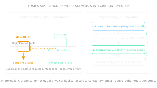
Every simulation step advances the physical world through four tightly coupled phases:

1. Forward Dynamics: Integrates the equations of motion (the Manipulator Equation): $$\mathbf{M}(\mathbf{q}) \ddot{\mathbf{q}} + \mathbf{C}(\mathbf{q}, \dot{\mathbf{q}})\dot{\mathbf{q}} + \mathbf{g}(\mathbf{q}) = \boldsymbol{\tau} + \mathbf{J}_c^T \mathbf{f}_c$$ where $\mathbf{M}$ is the inertia matrix, $\mathbf{C}$ captures Coriolis and centrifugal effects, $\mathbf{g}$ is gravity, $\boldsymbol{\tau}$ is motor torque, and $\mathbf{J}_c^T \mathbf{f}_c$ represents contact wrenches.
2. Collision Detection: Broadphase uses bounding volume hierarchies (BVH) to prune distant pairs; narrowphase uses algorithms like Gilbert-Johnson-Keerthi (GJK) and Expanding Polytope Algorithm (EPA) to determine contact points and penetration depths.
3. Contact Constraint Solving: Enforces non-penetration and Coulomb friction cones. Because rigid bodies cannot interpenetrate, contact is formulated as a Linear Complementarity Problem (LCP): $$0 \le d_n \perp f_n \ge 0$$ where $d_n$ is normal separation distance and $f_n$ is normal contact force. Either distance is zero (in contact, force $> 0$) or force is zero (separated, distance $> 0$).
4. Numerical Integration: Advances positions and velocities forward by timestep $\Delta t$ using Semi-Implicit Euler or Runge-Kutta integration: $$\dot{\mathbf{q}}_{t+1} = \dot{\mathbf{q}}_t + \Delta t \, \ddot{\mathbf{q}}_t$$ \mathbf{q}}_{t+1} = \mathbf{q}_t + \Delta t \, \dot{\mathbf{q}}_{t+1}

Timestep selection and penetration depth

In discrete simulation, continuous motion is evaluated at intervals $\Delta t$. If a rigid object moves at impact velocity $v_{\text{impact}}$ toward a surface, it moves a discrete distance $\Delta z = v_{\text{impact}} \Delta t$ during one step before collision detection runs.

In penalty-based contact models, restoring force is proportional to penetration: $F_{\text{contact}} = k \Delta z$. If $\Delta t$ is too large, the object penetrates deeply into the floor before the engine detects it. The resulting restoring force is artificially massive, injecting non-physical energy and causing objects to explode off the ground.

Worked example: contact penetration at 10 ms versus 1 ms

A rigid block falls toward a table, reaching an impact velocity $v_{\text{impact}} = 0.50\text{ m/s}$ ($50\text{ cm/s}$):

• Case 1: Large timestep $\Delta t_1 = 0.010\text{ s}$ ($10\text{ ms}$, typical for fast video games):

  $$\Delta z_1 = v_{\text{impact}} \times \Delta t_1 = 0.50 \times 0.010 = 0.0050\text{ m} = 5.0\text{ mm}$$

  The block sinks $5.0\text{ mm}$ into the solid table before the contact solver detects the collision. If surface stiffness $k = 10{,}000\text{ N/m}$, the restoring spring force spikes instantly to $F_1 = 10{,}000 \times 0.005 = 50\text{ N}$, kicking the block into an unphysical high-velocity bounce.

• Case 2: Tight integration timestep $\Delta t_2 = 0.001\text{ s}$ ($1\text{ ms}$, standard in robotics physics engines):

  $$\Delta z_2 = v_{\text{impact}} \times \Delta t_2 = 0.50 \times 0.001 = 0.0005\text{ m} = 0.5\text{ mm}$$

  The penetration is bounded to just $0.5\text{ mm}$ ($90\%$ reduction). The contact force remains smooth ($F_2 = 5\text{ N}$), allowing contact damping to dissipate kinetic energy naturally without explosive bouncing.

Code

This Python snippet simulates 1D discrete penalty contact integration under two different timesteps, calculating penetration depth, contact restoring force, and illustrating numerical stability.

1def simulate_impact_step(2    v_impact: float,3    dt: float,4    stiffness: float = 10000.0,5) -> tuple[float, float]:6    """Compute 1-step contact penetration (mm) and restoring force (N)."""7    penetration_m: float = v_impact * dt8    penetration_mm: float = penetration_m * 1000.09    restoring_force_n: float = stiffness * penetration_m10    return round(penetration_mm, 2), round(restoring_force_n, 1)11
12
13# Compare 10 ms timestep vs 1 ms timestep14pen_10ms, force_10ms = simulate_impact_step(v_impact=0.50, dt=0.010)15pen_1ms, force_1ms = simulate_impact_step(v_impact=0.50, dt=0.001)16
17print(pen_10ms)   # -> 5.018print(force_10ms)  # -> 50.019print(pen_1ms)    # -> 0.520print(force_1ms)   # -> 5.0

Watch Out For

The Quick Version

• Robot simulation enables parallel, accelerated, and risk-free data collection for reinforcement learning and policy verification.
• Physics engines approximate continuous dynamics through discrete numerical integration, collision detection, and contact complementarity solvers.
• An impact velocity of $0.50\text{ m/s}$ with a $10\text{ ms}$ timestep causes $5.0\text{ mm}$ of artificial penetration; cutting $\Delta t$ to $1\text{ ms}$ reduces penetration to $0.5\text{ mm}$.
• Photorealism is distinct from physical fidelity: accurate mass matrices, contact wrenches, and friction cones govern sim-to-real success before robot policy deployment to physical hardware.
• Decoupling high-frequency physics substeps ($1\text{ kHz}$) from policy decision steps ($50\text{ Hz}$) prevents numerical instability and simulator exploits.

What to Read Next

• Model Predictive Control for Robots
• Learning Robot Manipulation from Demonstrations
• Reinforcement Learning for Robot Control
• Deploying Robot Policies Across the Reality Gap