Robot Visual Servoing: Close the Image Loop

Look at the target again after moving. Use the remaining image error to choose the next camera motion instead of trusting a single reconstructed target pose.

Moving the camera right shifts a stationary feature left toward its desired image position.

Why Does This Exist?

An arm computes a target pose from one image and moves toward it. Small calibration or pose errors remain at the destination. Visual servoing closes feedback around visual measurements: observe features, compare them with a desired observation, compute motion and observe again. That correction can continue during approach.

A pinhole camera maps a point at $(X,Y,Z)$ in camera coordinates to normalized image coordinates $(x,y)=(X/Z,Y/Z)$ . Perception geometry explains this projection. Image-based visual servoing, or IBVS, uses such feature coordinates directly as its controlled output. Position-based visual servoing uses an estimated three-dimensional pose. This page derives the image-based velocity relationship; it does not replace joint tracking or a collision-free approach plan.

Think of It Like This

Centering a distant sign in a camera viewfinder

If a sign appears to the right of your desired position, shift the camera right without rotating it: the stationary sign moves left in the image. Look again and reduce the next shift as the sign approaches its mark. The image offset maps to feedback error, your hand motion to camera velocity, and repeated looks to the feedback cycle. The analogy stops when you rotate, approach or lose the sign; those motions change projection differently and require more than a horizontal rule.

How It Actually Works

What converts camera motion into feature motion?

For a stationary scene point and camera velocity $v_c=(v_x,v_y,v_z,\omega_x,\omega_y,\omega_z)^T$ , expressed in the camera frame, the interaction matrix is

\begin{bmatrix}\dot x\\\dot y\end{bmatrix} =L(x,y,Z)v_c,\qquad L=\begin{bmatrix} -1/Z&0&x/Z&xy&-(1+x^2)&y\\ 0&-1/Z&y/Z&1+y^2&-xy&-x \end{bmatrix}.

The $v$ components are linear speeds in m/s; the $\omega$ components are angular speeds in rad/s. Depth $Z>0$ is in metres. The rows follow by differentiating the projection and using point motion relative to a moving camera. The minus sign on $v_x$ is why camera-right motion produces image-left motion. Chaumette and Hutchinson's primary tutorial derives this matrix and discusses depth estimates, singularities and local convergence.

Stack feature coordinates into vector $s$ , desired coordinates into $s^*$ and their interaction matrices into $L_s$ . Error is $e=s-s^*$ . A common velocity request is $v_c=-\lambda\widehat L_s^+e$ , where $\lambda>0$ is a gain in inverse seconds, $+$ means pseudoinverse and the hat marks an estimated matrix. For a correctly modeled attainable error direction, this aims at $\dot e=-\lambda e$ . It is a local relationship: a pseudoinverse does not provide global convergence, joint feasibility or feature visibility.

Compute one lateral correction

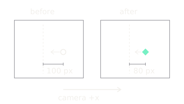
Restrict the camera to horizontal translation, hold scene depth at 1 m and set desired normalized horizontal coordinate to zero. Start at $x=0.2$ , so error is 0.2. With focal length $f_x=500$ pixels, pixel error is $500(0.2)=100$ pixels relative to the principal point. The scalar relation is $\dot x=-v_x/Z$ . Using $\lambda=2$ s⁻¹ and correct depth gives $v_x=\lambda Zx=0.4$ m/s rightward.

Hold that command for $h=0.1$ s. The camera translates 0.04 m right; the point's camera-relative horizontal coordinate drops from 0.2 to 0.16 m while depth stays 1 m. Hence normalized coordinate becomes 0.16 and pixel error becomes 80 pixels. The SVG uses identical image scales in both panels, with 0.7 drawing units per pixel. Dashed lines mark desired image coordinates; the mint diamond is the corrected feature. The bottom arrow is the camera command direction, not its physical displacement scale.

How wrong can the estimated depth be?

With depth estimate $\widehat Z$ and true depth $Z$ , the same restricted held-command update is

$x_{k+1}=\left(1-\lambda h\frac{\widehat Z}{Z}\right)x_k.$

Correct depth gives factor 0.8. Doubling estimated depth gives factor 0.6 and a larger correction; the loop can overshoot or diverge when the gain, sampling interval and depth ratio make the factor's magnitude at least one. In this ideal scalar case, decay requires $0<\lambda h\widehat Z/Z<2$ . This is not a stability criterion for general six-axis IBVS with delay, changing depth and joint saturation.

How does the camera request reach the arm?

Use hand-eye calibration to relate camera and tool motion. Transform the camera twist consistently, then map through the arm Jacobian or form a combined feature-to-joint Jacobian. Apply joint, velocity and visibility constraints inside that control design. Blindly clipping individual joints changes the feature motion predicted by $L_s$ .

One point supplies only two image constraints and cannot determine arbitrary six-component camera velocity. Multiple, well-distributed tracked features improve constraint coverage; even sufficient feature count can leave singular geometry or pose ambiguity. Damping bounds inverse amplification but trades tracking accuracy for restraint near weakly observed directions.

IBVS avoids requiring a full target pose at every update, but still needs reliable features, an interaction model and timely images. Position-based control can make workspace motion easier to interpret when pose is reliable, at the cost of dependence on that estimate. Use geometric planning for large unseen moves; reserve image correction for conditions where features remain visible and the local model is useful.

Code

This standalone Python repeats the restricted lateral update and checks it directly against geometric translation. It is an offline teaching model, not a robot driver.

1def lateral_step(x: float, depth: float, depth_estimate: float,2                 dt: float, gain: float) -> tuple[float, float]:3    if min(depth, depth_estimate, dt, gain) <= 0:4        raise ValueError("Depths, timestep and gain must be positive")5    speed = gain * depth_estimate * x6    point_x = x * depth - speed * dt7    return point_x / depth, speed8
9
10x = 0.211for _ in range(3):12    x, speed = lateral_step(x, 1.0, 1.0, 0.1, 2.0)13    print(f"camera {speed:.3f} m/s, pixel error {500*x:.2f}")14wrong, _ = lateral_step(0.2, 1.0, 12.0, 0.1, 2.0)15assert abs(wrong) > 0.216print(f"large depth error: {500*wrong:.2f} pixels")

The three lines give camera speeds 0.400, 0.320, 0.256 m/s and pixel errors 80.00, 64.00, 51.20. The excessive depth estimate gives -140.00 pixels: the feature crosses the target and the error magnitude grows.

Watch Out For

Image error grows after every correction

Check whether the commanded velocity describes the camera moving through the scene or the scene moving relative to the camera. For this convention, positive camera x produces negative feature x. Verify a small recorded motion and its measured image shift before increasing gain; a sign error cannot be tuned away.

A good image step is physically infeasible

Features approach their targets while joints saturate, the camera loses another feature or the tool approaches an obstacle. Model the camera-to-joint mapping and constraints together. Timestamp the exposure and reject stale features; feature-error reduction alone does not establish clearance or whole-body stability.

The Quick Version

Visual servoing repeatedly corrects motion from measured visual-feature error.
The interaction matrix maps camera twist to image-feature velocity and depends on geometry.
The worked rightward camera shift reduces the example error from 100 to 80 pixels.
Depth uncertainty, gain and sample interval jointly affect the correction.
Image convergence requires appropriate features and does not imply joint or collision feasibility.