Asynchronous Advantage Actor-Critic (A3C)
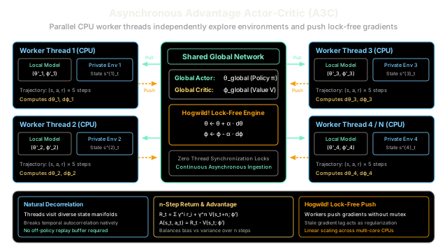
Asynchronous Advantage Actor-Critic runs parallel worker threads that independently explore environments and update a shared central model without locks, breaking data correlation without an off-policy replay buffer.
Why Does This Exist?
In early deep reinforcement learning, algorithms like Deep Q-Networks (DQN) relied on massive experience replay buffers (typically storing 1,000,000 transitions in memory) to break the temporal autocorrelation of sequential data. Without a replay buffer, training a neural network on consecutive states () causes weights to overfit to the agent's immediate trajectory, destabilizing learning.
However, experience replay introduced two critical bottlenecks:
- Incompatibility with On-Policy Methods: Replay memory inherently serves older transitions collected by past policies. On-policy policy gradient algorithms—such as standard Actor-Critic and REINFORCE—require trajectories sampled strictly from the current policy , making them unable to use experience replay without complex, variance-inducing importance sampling corrections.
- Severe Memory and Computational Overhead: Storing millions of high-dimensional raw pixel frames consumes gigabytes of RAM and demands specialized off-policy architectures.
In 2016, Mnih et al. introduced Asynchronous Advantage Actor-Critic (A3C) to solve temporal correlation without replay memory. Instead of storing past transitions from a single agent, A3C executes multiple parallel worker threads on a single multi-core CPU workstation. Because each worker interacts with its own private copy of the environment, different workers visit completely different regions of the state space simultaneously. When workers asynchronously push their local gradients to a shared central model, the resulting stream of parameter updates is naturally decorrelated, enabling stable, efficient on-policy learning at a fraction of the hardware cost.
Think of It Like This
Field Scouts Updating the Central Playbook
Imagine an athletic coaching staff preparing a master strategy playbook for an upcoming tournament:
- The Central Playbook (Global Shared Model): A master tactical playbook resides at headquarters containing current offensive plays () and defensive risk evaluations ().
- Parallel Field Scouts (Worker Threads): Instead of sending one scout to observe one team at a time, the coaching staff deploys four scouts to four different rival arenas simultaneously.
- Local Exploration & Strategy Testing: Each scout carries a copy of the morning playbook. Scout A watches an aggressive pressing team, Scout B watches a zone-defense team, and Scout C watches a fast-break team. Each scout tests tactics over a 5-minute stretch (-step trajectory).
- Asynchronous Dispatch (Lock-Free Push): Whenever a scout finishes evaluating their 5-minute drill, they immediately radio headquarters to dictate strategy adjustments. Headquarters updates the master playbook on the spot without placing other scouts on hold or waiting for all four scouts to finish at the exact same minute.
- Fresh Playbook Synchronization (Parameter Pull): Before launching their next 5-minute drill, each scout downloads the latest version of the master playbook.
Because the scouts observe completely different opponents in different cities, the stream of tactical feedback arriving at headquarters is diverse and balanced. Headquarters never overfits to a single opponent's playbook.
Where the analogy stops: Human dispatchers write notes one at a time. In A3C, worker threads apply their gradient updates directly to shared CPU memory using lock-free Hogwild! optimization. Multiple CPU threads occasionally overwrite individual weight floats simultaneously without mutex locks; in deep networks, this slight race-condition noise acts as benign stochastic regularization.
How It Actually Works
Parallel Actor-Critic Formulation and Asynchronous Lock-Free Optimization
A3C maintains a central global network parameterized by policy weights (the Actor) and value baseline weights (the Critic). It spawns worker threads, each maintaining local parameter copies and alongside an independent copy of the environment.
+-----------------------------------------------------------------------------------------+| A3C WORKER THREAD LIFECYCLE |+-----------------------------------------------------------------------------------------+| 1. Pull Parameters | θ' ← θ_global, ϕ' ← ϕ_global || 2. Local Rollout | Step private environment for t_max steps (s_0, a_0, r_1, ..., s_t)|| 3. Bootstrap Return | R = 0 if terminal, else R = V(s_t; ϕ') || 4. Compute n-Step | For i = t-1 down to 0: R ← r_i+1 + γ R; A_i = R - V(s_i; ϕ') || 5. Accumulate Grads | dθ += ∇ log π(a_i | s_i) A_i + β ∇ H(π); dϕ -= (R - V_i) ∇ V_i || 6. Push Gradients | θ_global ← θ_global + α dθ; ϕ_global ← ϕ_global - α dϕ (Lock-free)|+-----------------------------------------------------------------------------------------+1. The Local Worker Rollout and -Step Advantage
Each worker resets its accumulated local gradients , , synchronizes local weights with the global parameters, and interacts with its environment for up to steps (typically ).
The worker bootstraps the cumulative return from the final state:
Working backward from step down to , the cumulative -step discounted return and advantage estimate are computed as:
The -step advantage strikes an effective bias-variance tradeoff: multi-step rewards reduce the bias of the learned value critic, while bootstrapping from avoids the high variance of full Monte Carlo rollouts.
2. Gradient Accumulation with Entropy Regularization
The worker accumulates policy gradients, critic loss gradients, and an entropy regularization term:
where is policy entropy, and controls the exploration bonus that discourages premature convergence to deterministic policies.
3. Lock-Free Hogwild! Parameter Push
The worker applies its accumulated gradients directly to the shared global parameters:
These updates are performed asynchronously without thread mutex locks (the Hogwild! approach). Because different workers update the model at varying timestamps, a worker's gradients may be computed on slightly stale parameters (). In practice, as long as the number of parallel workers remains within reasonable bounds, this mild gradient staleness does not impede convergence.
4. The Transition from A3C to Synchronous A2C
A3C was conceived during the era of multi-core CPU computing. However, as deep learning hardware evolved, GPUs proved far more efficient at batched matrix multiplications than running independent threads.
This led to the development of Advantage Actor-Critic (A2C), the synchronous counterpart to A3C:
- Instead of asynchronous updates, A2C waits for all parallel workers to complete their steps.
- It pools the collected transitions into a single synchronized mini-batch ( samples) and executes a single batched GPU forward and backward pass.
- A2C matches or exceeds A3C's performance while utilizing GPU tensor cores efficiently and completely eliminating gradient staleness.
Worked numerical example
Let us trace a concrete 2-worker asynchronous parameter update scenario tracking a shared 2-dimensional parameter vector .
1. Initial State
- Shared global parameters: .
- Step size (learning rate): .
- Both Worker 1 and Worker 2 initialize by pulling the global parameters:
2. Worker 1 Execution (Fast Rollout)
Worker 1 runs a short 1-step trajectory in Environment 1. It evaluates its local objective and computes gradient vector :
Worker 1 pushes to the global parameter store:
Worker 1 finishes its cycle and pulls the updated parameters: .
3. Worker 2 Execution (Slower Rollout with Stale Parameters)
Meanwhile, Worker 2 was executing a longer 3-step rollout in Environment 2. During this time, Worker 2 still held its local parameters .
Worker 2 computes its accumulated trajectory gradient based on its local parameters:
Notice that is a stale gradient because the global model has already progressed to .
4. Asynchronous Push by Worker 2
Under Hogwild! semantics, Worker 2 does not discard its gradient; it writes directly to the shared global memory without acquiring locks:
Worker 2 then pulls the fresh global model:
Despite the 1-update staleness, Worker 2 contributed valid directional information that guided parameters toward the joint multi-environment objective.
Code
The following self-contained Python script implements a multi-threaded A3C simulation where parallel worker threads explore independently and update a central SharedGlobalModel asynchronously without locks.
import threadingimport timefrom typing import Listimport numpy as np
class SharedGlobalModel: """Central parameter store updated asynchronously by worker threads without locks."""
def __init__(self, dim: int = 2, lr: float = 0.05) -> None: self.params = np.zeros(dim, dtype=np.float64) self.lr = lr self.update_count = 0
def apply_gradients(self, grads: np.ndarray) -> None: """Lock-free asynchronous parameter update (Hogwild! style).""" self.params -= self.lr * grads self.update_count += 1
def get_params(self) -> np.ndarray: """Pull a copy of current global parameters.""" return self.params.copy()
class A3CWorker(threading.Thread): """Local worker thread interacting with a private environment copy."""
def __init__( self, worker_id: int, global_model: SharedGlobalModel, target_optimum: np.ndarray, num_steps: int = 40, delay_ms: float = 0.001, ) -> None: super().__init__() self.worker_id = worker_id self.global_model = global_model self.target = target_optimum self.num_steps = num_steps self.delay_ms = delay_ms self.local_params = global_model.get_params() self.gradients_pushed = 0
def run(self) -> None: for _ in range(self.num_steps): # 1. Pull latest global parameters self.local_params = self.global_model.get_params()
# 2. Simulate local environment interaction and gradient computation # Objective: minimize 0.5 * ||params - target||^2 -> grad = params - target grad = self.local_params - self.target # Add stochastic exploration noise unique to this environment instance grad += np.random.normal(0.0, 0.02, size=grad.shape)
time.sleep(self.delay_ms)
# 3. Push gradient asynchronously to global shared model self.global_model.apply_gradients(grad) self.gradients_pushed += 1
if __name__ == "__main__": # 1. Verify Worked Numerical Trace (2 workers, deterministic) shared = SharedGlobalModel(dim=2, lr=0.10) shared.params = np.array([1.00, 2.00], dtype=np.float64)
# Worker 1 push g1 = np.array([0.40, -0.60]) shared.apply_gradients(g1) print("=== Worked Numerical Trace ===") print("Global params after Worker 1 push:", np.round(shared.params, 4)) assert np.allclose(shared.params, [0.96, 2.06])
# Worker 2 push (stale gradient computed on [1.00, 2.00]) g2 = np.array([-0.50, 0.30]) shared.apply_gradients(g2) print("Global params after Worker 2 push:", np.round(shared.params, 4)) assert np.allclose(shared.params, [1.01, 2.03])
# 2. Multi-Threaded Asynchronous Execution Simulation target = np.array([3.0, -1.5]) async_global = SharedGlobalModel(dim=2, lr=0.08) async_global.params = np.array([0.0, 0.0], dtype=np.float64)
num_workers = 3 steps_per_worker = 40 workers = [ A3CWorker( worker_id=i, global_model=async_global, target_optimum=target, num_steps=steps_per_worker, delay_ms=0.001 * (i + 1), ) for i in range(num_workers) ]
print("\n=== Launching 3 Asynchronous Worker Threads ===") for w in workers: w.start() for w in workers: w.join()
final_params = async_global.get_params() total_updates = async_global.update_count print(f"All worker threads completed. Total updates: {total_updates}") print(f"Target Optimum : {target}") print(f"Converged Params: {np.round(final_params, 4)}")
# Verification assertions assert total_updates == num_workers * steps_per_worker assert np.allclose(final_params, target, atol=0.15) print("\nAll assertions passed successfully!")
# Expected Output:# === Worked Numerical Trace ===# Global params after Worker 1 push: [0.96 2.06]# Global params after Worker 2 push: [1.01 2.03]## === Launching 3 Asynchronous Worker Threads ===# All worker threads completed. Total updates: 120# Target Optimum : [ 3. -1.5]# Converged Params: [ 2.9958 -1.5022]## All assertions passed successfully!Watch Out For
Gradient Staleness and Destructive Overwrites
A3C assumes that local worker gradients remain useful despite being computed on slightly delayed parameter snapshots.
The Failure Mode: When scaling to high thread counts (e.g., 32 or 64 threads on high-core CPUs) or when environment instances have widely varying episode durations, worker latency diverges significantly. A slow worker may spend 200 milliseconds finishing an episode, by which time faster threads have updated the global network 150 times. Applying this deeply stale gradient pushes the global parameters along an obsolete loss surface direction, causing sudden catastrophic performance degradation or parameter divergence.
The Fix:
- Calibrate Worker Count: Keep the number of active worker threads strictly bounded to the physical core count (typically 8 to 16 threads).
- Adaptive Optimizers with Shared Statistics: Use Shared RMSprop or Shared Adam, which maintain running moving averages of squared gradients across all workers, dampening the impact of anomalous stale gradients.
- Transition to Synchronous A2C: If running on modern GPU hardware, migrate to synchronous A2C or batched PPO, which completely eliminates gradient staleness by synchronizing environment steps before computing backpropagation.
The Quick Version
- Natural Decorrelation: A3C breaks temporal autocorrelation by running multiple parallel CPU threads across private environment copies, eliminating the need for an off-policy replay buffer.
- On-Policy Advantage Actor-Critic: Each worker collects -step trajectories, bootstraps returns using a learned value critic , and updates the policy via advantage-weighted policy gradients with entropy regularization.
- Hogwild! Lock-Free Updates: Workers push accumulated gradients directly to the shared global model without thread mutex locks, maximizing multi-core CPU throughput.
- A3C to A2C Evolution: While A3C revolutionized multi-core CPU training, synchronous A2C superseded it on GPUs by batching parallel rollouts into efficient vectorized tensor operations.