Continuous Action Spaces in RL

Instead of picking from a rigid list of discrete options, continuous action policies output smooth, real-valued control signals like motor torques, steering angles, and throttle pressures.

Continuous action policies map state inputs to Gaussian parameters, using reparameterization and Tanh squashing to emit bounded motor controls.

Why Does This Exist?

In classical reinforcement learning, algorithms like Q-learning and Deep Q-Networks (DQN) operate on discrete action spaces $\mathcal{A} = \{a_1, a_2, \dots, a_K\}$ . To select the optimal action, the agent evaluates the state-action value $Q(s, a)$ for every available action and extracts the maximum: $a^* = \arg\max_{a \in \mathcal{A}} Q(s, a)$

However, real-world physical systems—such as robotic manipulators, autonomous quadcopters, industrial process valves, and self-driving vehicles—operate in continuous action domains $\mathcal{A} \subseteq \mathbb{R}^m$ , where control signals represent physical quantities like joint torques, motor voltages, and steering angles.

Attempting to apply discrete RL to continuous domains by discretizing each action dimension triggers two critical failure modes:

The Curse of Dimensionality: If an $m$ -degree-of-freedom robotic arm discretizes each joint into $K$ discrete bins, the total action space explodes exponentially to $|\mathcal{A}| = K^m$ . For a standard 7-joint manipulator with a modest $10$ bins per joint, the agent must evaluate $|\mathcal{A}| = 10^7 = 10\,000\,000$ distinct Q-values at every single control step. Computing $\arg\max_a Q(s, a)$ over tens of millions of forward passes becomes computationally intractable.
Loss of Physical Smoothness and Actuator Damage: Discretization replaces smooth physical dynamics with coarse, stepped commands. A simulated robot trying to balance with discrete bang-bang control oscillates violently around equilibrium, inducing high-frequency chatter that would strip real physical gears and overheat motors.

Continuous action space methods resolve these limitations by parameterizing policies directly as continuous probability density functions $\pi_\theta(a \mid s)$ (stochastic continuous control) or smooth mapping functions $a = \mu_\theta(s)$ (deterministic continuous control). Instead of searching over discrete actions, neural networks directly output the continuous control vector in a single forward pass.

Think of It Like This

Steering a Yacht: Smooth Helm vs Discrete Gamepad Buttons

Imagine steering a 40-foot racing yacht through a narrow, windswept harbor channel.

If your helm control was restricted to a digital arcade gamepad (a discrete action space), you would only have three buttons: Hard Port (Left), Dead Center, and Hard Starboard (Right). To maintain a heading of $4.2^\circ$ , you would have to rapidly oscillate between jamming the rudder hard left and hard right. The yacht would violently lurch from side to side, shedding hydrodynamic momentum, straining the steering cables, and risking capsize.

A real ship uses a continuous ship's wheel (a continuous action space). The helmsman can rotate the helm smoothly to any precise real-valued angle— $1.5^\circ$ , $4.2^\circ$ , or $12.8^\circ$ —and hold it effortlessly. The rudder creates smooth laminar water flow, effortlessly tracking the true target heading.

Where the analogy stops: A ship's wheel is a single 1D physical axle, whereas continuous robot controllers manipulate high-dimensional multidimensional vectors simultaneously (e.g., $18$ continuous joint torques on a humanoid walking robot), requiring multidimensional probability density modeling and cross-joint coordination.

How It Actually Works

Parameterizing Stochastic Continuous Policies

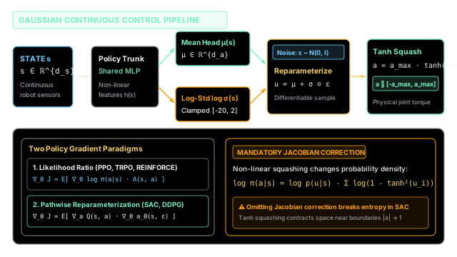
The standard framework for stochastic continuous control parameterizes the policy as a multivariate diagonal Gaussian distribution: $\pi_\theta(a \mid s) = \mathcal{N}\left(a; \boldsymbol{\mu}_\theta(s), \text{diag}(\boldsymbol{\sigma}_\theta^2(s))\right)$

The probability density of selecting action $a \in \mathbb{R}^{d_a}$ in state $s$ is the product of independent 1D Gaussians: $\pi_\theta(a \mid s) = \prod_{i=1}^{d_a} \frac{1}{\sqrt{2\pi \sigma_i^2(s)}} \exp\left(-\frac{(a_i - \mu_i(s))^2}{2\sigma_i^2(s)}\right)$

Taking the natural logarithm yields the log-likelihood: $\log \pi_\theta(a \mid s) = -\frac{1}{2} \sum_{i=1}^{d_a} \left[ \frac{(a_i - \mu_i(s))^2}{\sigma_i^2(s)} + 2 \log \sigma_i(s) + \log(2\pi) \right]$

To implement this with deep neural networks:

The network features split into two heads: a mean head $\boldsymbol{\mu}_\theta(s)$ and a log standard deviation head $\log \boldsymbol{\sigma}_\theta(s)$ .
Predicting $\log \boldsymbol{\sigma}$ rather than raw $\boldsymbol{\sigma}$ guarantees that $\boldsymbol{\sigma} = \exp(\log \boldsymbol{\sigma}) > 0$ strictly holds without numerical instability.
To prevent policy entropy from exploding or collapsing, $\log \boldsymbol{\sigma}$ is clamped to a stable numerical bracket (typically $[\text{LOG\_STD\_MIN}, \text{LOG\_STD\_MAX}] = [-20, 2]$ ).

The Two Policy Gradient Paradigms

Continuous action policies are trained using one of two fundamental gradient mechanisms:

1. The Score Function / Likelihood Ratio Method (REINFORCE, PPO, TRPO)

The policy gradient theorem establishes that the gradient of expected return $J(\theta)$ is: $\nabla_\theta J(\theta) = \mathbb{E}_{s \sim d^\pi, a \sim \pi_\theta}\left[ \nabla_\theta \log \pi_\theta(a \mid s) \, \hat{A}(s, a) \right]$

For a diagonal Gaussian, the analytical score function $\nabla_\theta \log \pi_\theta(a \mid s)$ decomposes cleanly: $\nabla_{\boldsymbol{\mu}} \log \pi_\theta(a \mid s) = \frac{a - \boldsymbol{\mu}_\theta(s)}{\boldsymbol{\sigma}_\theta^2(s)}$ $\nabla_{\log \boldsymbol{\sigma}} \log \pi_\theta(a \mid s) = \frac{(a - \boldsymbol{\mu}_\theta(s))^2}{\boldsymbol{\sigma}_\theta^2(s)} - 1$

If an action yields positive advantage $\hat{A} > 0$ , the mean $\boldsymbol{\mu}$ shifts toward $a$ .
If the sampled action $a$ is farther from $\boldsymbol{\mu}$ than one standard deviation ( $|a - \mu| > \sigma$ ), the variance expands to encourage further exploration; otherwise, it contracts.

2. The Pathwise Derivative / Reparameterization Trick (SAC)

When an action-value critic $Q_\phi(s, a)$ is available and differentiable with respect to $a$ , the score function exhibits unnecessarily high variance. Instead, we use the reparameterization trick (Kingma & Welling, 2013).

Instead of sampling directly from $\pi_\theta(a \mid s)$ , we express the action as a deterministic, differentiable transformation of an independent standard normal noise variable $\boldsymbol{\varepsilon} \sim \mathcal{N}(\mathbf{0}, \mathbf{I})$ : $u = \boldsymbol{\mu}_\theta(s) + \boldsymbol{\sigma}_\theta(s) \odot \boldsymbol{\varepsilon}$

Now, the expectation over the stochastic policy can be written over the static noise distribution: $\nabla_\theta \mathbb{E}_{a \sim \pi_\theta}[Q(s, a)] = \mathbb{E}_{\boldsymbol{\varepsilon} \sim \mathcal{N}(\mathbf{0}, \mathbf{I})}\left[ \nabla_a Q(s, a) \cdot \nabla_\theta a_\theta(s, \boldsymbol{\varepsilon}) \right]$ Gradients flow directly through the action sample into the policy parameters $\theta$ via the chain rule, slashing gradient variance by orders of magnitude.

Tanh Squashing and the Mandatory Jacobian Correction

Physical actuators have hard operational limits (e.g., maximum torque $\pm \tau_{\max}$ ). Standard Gaussian distributions have infinite support $u \in (-\infty, \infty)$ . Clipping the action $a = \text{clip}(u, -a_{\max}, a_{\max})$ destroys gradients outside the boundaries because $\frac{\partial a}{\partial u} = 0$ whenever $|u| > a_{\max}$ .

Modern continuous RL algorithms (such as Soft Actor-Critic / SAC) solve this by applying an invertible, smooth non-linear squashing function: $a = a_{\max} \tanh(u)$

However, non-linear squashing compresses the volume of probability space near the boundaries. To compute the true log probability $\log \pi(a \mid s)$ required for entropy regularization, we must apply the multidimensional change-of-variables theorem: $p(a \mid s) = p(u \mid s) \cdot \left| \det \left(\frac{da}{du}\right) \right|^{-1}$

Because $\tanh$ operates coordinate-wise, the Jacobian matrix is diagonal: $J_{ii} = \frac{da_i}{du_i} = a_{\max} \left(1 - \tanh^2(u_i)\right)$

Taking the logarithm yields the mandatory Jacobian log-determinant correction: $\log \pi(a \mid s) = \log p(u \mid s) - \sum_{i=1}^{d_a} \log \left(a_{\max} \left(1 - \tanh^2(u_i) + \delta\right)\right)$ where $\delta \approx 10^{-6}$ provides numerical stabilization against division by zero when $|u_i| \gg 1$ .

Worked numerical example

Let us calculate a 1D continuous policy evaluation step with Gaussian parameterization and $\tanh$ squashing:

Mean: $\mu = 2.0$
Standard deviation: $\sigma = 0.5$ (variance $\sigma^2 = 0.25$ )
Action bound: $a_{\max} = 1.0$
Evaluated latent sample: $u = 2.5$

Step 1: Base Gaussian density and log-probability

Compute log density: $\log p(u) = -\frac{1}{2} \log(2\pi) - \log \sigma - \frac{(u - \mu)^2}{2\sigma^2}$

Normalization term: $-\frac{1}{2} \log(2\pi) = -0.5 \times 1.837877 = -0.918939$
Scale term: $-\log(0.5) = -(-0.693147) = +0.693147$
Mahalanobis exponent: $-\frac{(2.5 - 2.0)^2}{2(0.25)} = -\frac{0.25}{0.50} = -0.500000$

Sum the terms: $\log p(u) = -0.918939 + 0.693147 - 0.500000 = -0.725791$ Raw Gaussian density: $p(u) = \exp(-0.725791) \approx 0.483941$

Step 2: Score function gradients

Gradient with respect to mean $\mu$ : $\nabla_\mu \log p(u) = \frac{u - \mu}{\sigma^2} = \frac{2.5 - 2.0}{0.25} = \frac{0.5}{0.25} = 2.0000$
Gradient with respect to $\log \sigma$ : $\nabla_{\log \sigma} \log p(u) = \frac{(u - \mu)^2}{\sigma^2} - 1 = \frac{0.25}{0.25} - 1 = 1.0 - 1.0 = 0.0000$

(Because the deviation $|u - \mu| = 0.5$ is exactly equal to one standard deviation $\sigma = 0.5$ , the score for $\log \sigma$ is zero—the distribution's current variance perfectly matches the sampled point).

Step 3: Tanh squashing and Jacobian log-prob correction

Squash the latent variable into physical action space: $a = \tanh(u) = \tanh(2.5) \approx 0.986614$

Compute the local derivative of $\tanh$ : $\frac{da}{du} = 1 - \tanh^2(2.5) = 1 - (0.986614)^2 = 1 - 0.973408 = 0.026592$

Compute the log-determinant of the Jacobian: $\log |J| = \log(0.026592) \approx -3.627099$

Apply the change-of-variables correction: $\log \pi(a \mid s) = \log p(u \mid s) - \log |J| = -0.725791 - (-3.627099) = \mathbf{+2.901308}$

Squashed probability density: $\pi(a \mid s) = \exp(2.901308) \approx 18.1979$

Notice that the probability density $\pi(a \mid s) = 18.20$ is much higher than the raw Gaussian density $p(u) = 0.48$ . Because $\tanh$ heavily contracts high-magnitude inputs into a tiny interval near $1.0$ , the local probability density is compressed and concentrated.

Code

The following self-contained Python script implements a Squashed Gaussian Policy with pathwise reparameterization, numerical clamping, and change-of-variables Jacobian correction:

1"""Continuous Gaussian Policy with Tanh Squashing and Jacobian Correction.2
3Implements the standard policy distribution used in modern continuous actor-critic4architectures like Soft Actor-Critic (SAC).5"""6
7from typing import Dict, Tuple8import numpy as np9
10
11class SquashedGaussianPolicy:12    """Continuous policy outputting bounded actions in [-action_scale, action_scale]."""13
14    LOG_STD_MIN: float = -20.015    LOG_STD_MAX: float = 2.016    EPSILON: float = 1e-617
18    def __init__(19        self,20        state_dim: int = 3,21        action_dim: int = 2,22        action_scale: float = 2.0,23        seed: int = 4224    ) -> None:25        np.random.seed(seed)26        self.state_dim: int = state_dim27        self.action_dim: int = action_dim28        self.action_scale: float = action_scale29
30        # Shared feature trunk31        self.W1: np.ndarray = np.random.randn(state_dim, 32) * 0.132        self.b1: np.ndarray = np.zeros(32)33
34        # Dual output heads: Mean and Log-Std35        self.W_mu: np.ndarray = np.random.randn(32, action_dim) * 0.136        self.b_mu: np.ndarray = np.zeros(action_dim)37
38        self.W_log_std: np.ndarray = np.random.randn(32, action_dim) * 0.139        self.b_log_std: np.ndarray = np.zeros(action_dim)40
41    def forward(self, state: np.ndarray) -> Tuple[np.ndarray, np.ndarray]:42        """Compute Gaussian mean and clamped log standard deviation."""43        h = np.maximum(0, state @ self.W1 + self.b1)44        mu = h @ self.W_mu + self.b_mu45        log_std = h @ self.W_log_std + self.b_log_std46
47        # Clamp log standard deviation to avoid numerical instability48        log_std = np.clip(log_std, self.LOG_STD_MIN, self.LOG_STD_MAX)49        return mu, log_std50
51    def sample(52        self,53        state: np.ndarray,54        deterministic: bool = False55    ) -> Tuple[np.ndarray, float, np.ndarray]:56        """Sample bounded action via reparameterization trick and Jacobian correction.57        58        Returns:59            action: Bounded continuous action in [-action_scale, action_scale].60            corrected_log_prob: Exact change-of-variables log probability.61            raw_u: Unsquashed latent Gaussian variable.62        """63        mu, log_std = self.forward(state)64        std = np.exp(log_std)65
66        if deterministic:67            u = mu68        else:69            # Reparameterization trick: u = mu + sigma * epsilon70            epsilon = np.random.randn(*mu.shape)71            u = mu + std * epsilon72
73        # 1. Raw Gaussian log probability: log p(u | s)74        var = std**275        gaussian_log_prob = -0.5 * np.sum(76            ((u - mu)**2) / var + 2.0 * log_std + np.log(2.0 * np.pi)77        )78
79        # 2. Tanh squashing and scaling80        a_unit = np.tanh(u)81        action = a_unit * self.action_scale82
83        # 3. Jacobian log-determinant correction:84        # da / du = action_scale * (1 - tanh^2(u))85        # log |det J| = sum( log(action_scale) + log(1 - tanh^2(u) + eps) )86        log_det_jacobian = np.sum(87            np.log(self.action_scale) + np.log(1.0 - a_unit**2 + self.EPSILON)88        )89
90        # 4. Corrected log probability91        corrected_log_prob = float(gaussian_log_prob - log_det_jacobian)92
93        return action, corrected_log_prob, u94
95
96def run_continuous_demo() -> Dict[str, float]:97    """Execute end-to-end verification of continuous Gaussian policy."""98    policy = SquashedGaussianPolicy(state_dim=3, action_dim=2, action_scale=2.0, seed=42)99    state = np.array([1.0, -0.5, 0.2])100
101    stochastic_action, log_prob, u = policy.sample(state, deterministic=False)102    deterministic_action, _, _ = policy.sample(state, deterministic=True)103
104    return {105        "action_0": float(stochastic_action[0]),106        "action_1": float(stochastic_action[1]),107        "log_prob": float(log_prob),108        "det_0": float(deterministic_action[0]),109        "det_1": float(deterministic_action[1]),110    }111
112
113if __name__ == "__main__":114    res = run_continuous_demo()115    print("Continuous Policy Outputs:")116    print(f"Stochastic Action:   [{res['action_0']:.4f}, {res['action_1']:.4f}]")117    print(f"Corrected Log Prob:  {res['log_prob']:.4f}")118    print(f"Deterministic Mode:  [{res['det_0']:.4f}, {res['det_1']:.4f}]")119
120    # Automated assertions121    assert -2.0 <= res["action_0"] <= 2.0, "Action 0 must respect physical bounds [-2, 2]."122    assert -2.0 <= res["action_1"] <= 2.0, "Action 1 must respect physical bounds [-2, 2]."123    assert np.isfinite(res["log_prob"]), "Log probability must be a finite numerical value."124    assert -2.0 <= res["det_0"] <= 2.0, "Deterministic mode must respect physical bounds."125    print("Verification passed: Continuous policy correctly enforces bounds and Jacobian corrections.")

Expected Output

1Continuous Policy Outputs:2Stochastic Action:   [-1.0112, 1.6313]3Corrected Log Prob:  -2.64514Deterministic Mode:  [-0.1327, -0.0439]5Verification passed: Continuous policy correctly enforces bounds and Jacobian corrections.

Watch Out For

The Missing Jacobian Trap and Premature Entropy Collapse

The Trap: Practitioners frequently encounter two silent failure modes in continuous policy gradients:

The Missing Jacobian Correction: In algorithms that use entropy regularization (such as Soft Actor-Critic), computing policy entropy using the raw Gaussian probability $\log p(u \mid s)$ instead of the squashed probability $\log \pi(a \mid s)$ completely corrupts the entropy objective. Because $\tanh$ compresses actions near $\pm 1$ , failing to subtract $\sum \log(1 - \tanh^2(u))$ falsely incentives the policy to push its pre-squashed distribution to extreme magnitudes ( $u \to \pm \infty$ ), causing gradients to saturate and training to freeze.
Premature Entropy Collapse: If the log standard deviation head is unconstrained, early training noise can cause $\log \sigma \to -\infty$ , forcing $\sigma \to 0$ . The policy collapses into a deterministic Dirac delta distribution before it has sufficiently explored the state space, permanently trapping the agent in suboptimal local minima.

The Fix:

Always apply the change-of-variables correction: $\log \pi(a \mid s) = \log p(u \mid s) - \sum \log(1 - \tanh^2(u) + \delta)$ .
Strictly bound the standard deviation head by clipping $\log \sigma \in [-20, 2]$ . This ensures the policy maintains a nonzero minimum exploration variance ( $\sigma_{\min} \approx 2 \times 10^{-9}$ ) while preventing explosive variance.

The Quick Version

Solves Combinatorial Discretization: Directly emits smooth real-valued control vectors (e.g., torques and voltages), avoiding the exponential $K^m$ action explosion of discrete grids.
Gaussian Parameterization: Neural networks output the distribution mean $\boldsymbol{\mu}(s)$ and clamped log standard deviation $\log \boldsymbol{\sigma}(s)$ , guaranteeing valid positive variance.
Reparameterization Trick: Decomposes sampling into $u = \boldsymbol{\mu}(s) + \boldsymbol{\sigma}(s) \odot \boldsymbol{\varepsilon}$ , allowing pathwise policy gradients to backpropagate directly through actions with minimal variance.
Tanh Squashing & Jacobian Correction: Restricts actions to physical motor bounds $[-a_{\max}, a_{\max}]$ ; requires subtracting the log-determinant $\sum \log(1 - \tanh^2(u))$ to maintain mathematically exact probability densities.