Equivalence of Forward and Backward Views
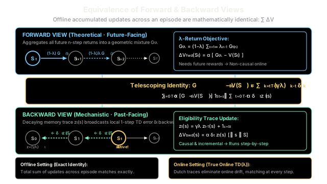
The forward view asks where future rewards will come from, while the backward view asks which past actions deserve credit for current rewards. Offline across an episode, these two fundamentally different perspectives produce the exact same mathematical updates.
Why Does This Exist?
In reinforcement learning theory, the forward view of is philosophically compelling: it defines an ideal learning target, the -return , by blending all future -step returns into a geometric mixture. However, the forward view is non-causal and acausal online—an agent standing at time cannot compute because it requires rewards and states that have not yet occurred.
To implement learning in real time, practitioners rely on the backward view: a mechanistic algorithm that looks backward into the past using an eligibility trace vector . Whenever a local one-step prediction error occurs, it broadcasts that error backward to recently visited states.
This introduces a foundational theoretical question: Are these two formulations actually solving the same problem?
The mathematical equivalence between the forward view and backward view proves that the mechanistic, step-by-step backward algorithm is not merely an intuitive heuristic. In the offline setting (when updates are accumulated and applied at the end of an episode), the sum of all backward updates across the trajectory is mathematically identical to the sum of all theoretical forward-view updates.
Think of It Like This
Two Ways to Audit Corporate Books
Imagine two different accountants auditing an enterprise's machinery expenditure across a fiscal year:
- The Forward-Looking Auditor (Forward View): At the moment a machine is purchased in January, this auditor projects forward across the machine's entire lifetime. They examine future maintenance bills, expected salvage value, and discounted utility to write an idealized depreciation entry for January. However, this auditor cannot finalize their books until the end of the year, after all actual receipts have been collected.
- The Daily Expense Clerk (Backward View): Each afternoon, the clerk records the actual bills that arrived today. If an unexpected repair bill arrives in October, the clerk does not travel back in time to change the January books. Instead, they write an immediate variance voucher, look at their ledger of currently active machinery, and distribute the expense backward across all active equipment.
At year-end, both accountants compute their bottom line:
- The forward auditor updated past purchases using total lifetime trajectories.
- The backward clerk updated daily books using local surprises broadcast across running inventories.
The result: Both methods arrive at the exact same fiscal balance. Where the analogy stops is that human accounting often deals with discrete legal tax categories, whereas in , the equivalence is established by an exact geometric decay factor that telescopes across every time step.
How It Actually Works
The Telescoping Sum Decomposition of the λ-Return
Let an episode terminate at step . At each step , the standard one-step Temporal Difference error is:
Now consider the sequence of -step returns starting from time :
- -step return:
- -step return:
- -step return:
Notice that the difference between any -step return and the initial value estimate expands into a telescoping sum of one-step TD errors:
In general, for any horizon :
The forward-view -return blends all -step returns geometrically with weights :
Subtracting from both sides and substituting the telescoping expansion, the geometric weights group each into an exponential factor:
This identity reveals that the forward -error is equal to the discounted sum of all future one-step TD errors from time to the end of the episode.
Swapping Summations: From Lookahead to Eligibility Traces
In the offline forward view, the value function is held fixed throughout the episode, and the total update applied to state at episode termination is the sum of forward updates over all visits:
This expression features a double summation over indices . Reversing the order of summation—making the outer loop over time steps and the inner loop over past visits:
Inspect the inner summation closely:
This matches the recursive definition of the accumulating eligibility trace:
Substituting directly back into the reversed summation gives:
This proves the exact offline equivalence: the forward view's future lookahead and the backward view's memory traces generate the identical cumulative weight update.
Worked numerical example
Consider a 2-step episodic trajectory:
Hyperparameters:
- Initial estimates: , .
- Discount factor , decay parameter , learning rate .
- Effective trace decay: .
1. Forward View Calculation
At step for state :
- 1-step return:
- 2-step full return:
- -return:
- Forward update for :
At step for state :
- Full return to terminal:
- -return:
- Forward update for :
2. Backward View Calculation
One-step TD errors:
Eligibility trace vector across steps ():
- Step : Visit
- Step : Decay by , visit
Accumulated backward updates:
- For state :
- For state :
The offline forward updates and offline backward updates match identically to three decimal places.
Offline Equivalence vs. Online Drift and True Online TD(λ)
The mathematical derivation above assumes that value estimates remain frozen while accumulating updates until the episode ends. When practitioners run standard online , value estimates are updated immediately after every transition:
Because changes on the fly, subsequent prediction errors are computed using rather than . This causes standard online to drift away from the forward-view -return, especially under large learning rates .
To resolve this discrepancy, van Seijen and Sutton (2014) introduced True Online . By employing Dutch traces:
and maintaining an auxiliary tracking scalar, True Online achieves exact step-by-step equivalence to the forward view in an online, causal algorithm—strictly dominating standard across tabular and linear approximation benchmarks.
Code
import mathfrom typing import Dict, List, Tuple
def verify_forward_backward_equivalence( trajectory: List[Tuple[str, float]], initial_values: Dict[str, float], gamma: float = 0.9, lam: float = 0.7, alpha: float = 0.1,) -> Tuple[Dict[str, float], Dict[str, float]]: """Compute and verify offline forward and backward TD(lambda) updates.
Args: trajectory: Sequence of (state, reward) pairs ending in 'terminal'. initial_values: Initial state-value mapping V_0(s). gamma: Discount factor in [0, 1]. lam: Trace decay parameter lambda in [0, 1]. alpha: Learning rate step size.
Returns: Tuple of (forward_updates, backward_updates) dictionaries. """ states = [s for s, _ in trajectory[:-1]] t_max = len(states) unique_states = sorted(list(set(states)))
# --------------------------------------------------------- # 1. Offline Forward View: Compute lambda-return G_t^lambda # --------------------------------------------------------- fwd_updates: Dict[str, float] = {s: 0.0 for s in unique_states}
for t in range(t_max): s_t = states[t] # Collect all n-step returns from step t n_step_returns: List[float] = [] for n in range(1, t_max - t + 1): # Sum discounted rewards up to step t + n return_val = 0.0 for i in range(n): reward_step = trajectory[t + i + 1][1] return_val += (gamma**i) * reward_step
# Add bootstrapped terminal value of horizon next_state = trajectory[t + n][0] if next_state != "terminal": return_val += (gamma**n) * initial_values[next_state] n_step_returns.append(return_val)
# Blend n-step returns with geometric weights (1 - lambda)*lambda^(n-1) g_lambda = 0.0 for n_idx, g_n in enumerate(n_step_returns[:-1]): weight = (1.0 - lam) * (lam**n_idx) g_lambda += weight * g_n
# Final term receives remaining geometric tail weight lambda^(H-1) last_weight = lam ** (len(n_step_returns) - 1) g_lambda += last_weight * n_step_returns[-1]
# Accumulate offline forward update fwd_updates[s_t] += alpha * (g_lambda - initial_values[s_t])
# --------------------------------------------------------- # 2. Offline Backward View: Accumulating Eligibility Traces # --------------------------------------------------------- bwd_updates: Dict[str, float] = {s: 0.0 for s in unique_states} traces: Dict[str, float] = {s: 0.0 for s in unique_states}
for t in range(t_max): s_t = states[t] next_s, r_t1 = trajectory[t + 1]
# Decay traces and bump visited state for s in traces: traces[s] *= gamma * lam traces[s_t] += 1.0
# One-step TD error using initial values next_v = 0.0 if next_s == "terminal" else initial_values[next_s] delta_t = r_t1 + gamma * next_v - initial_values[s_t]
# Accumulate backward update across all states for s in bwd_updates: bwd_updates[s] += alpha * delta_t * traces[s]
return fwd_updates, bwd_updates
if __name__ == "__main__": # Trajectory: S0 ->(R=3)-> S1 ->(R=4)-> terminal episode: List[Tuple[str, float]] = [ ("S0", 0.0), ("S1", 3.0), ("terminal", 4.0), ] v_init: Dict[str, float] = {"S0": 1.0, "S1": 2.0}
fwd, bwd = verify_forward_backward_equivalence( episode, v_init, gamma=0.9, lam=0.7, alpha=0.1 )
print("=== Verification of Forward-Backward Equivalence ===") for state in sorted(fwd.keys()): f_val = fwd[state] b_val = bwd[state] is_equal = math.isclose(f_val, b_val, rel_tol=1e-9) print( f"State {state} | Forward Delta V: {f_val:.6f} | " f"Backward Delta V: {b_val:.6f} | Exact Match: {is_equal}" ) assert is_equal, f"Mismatch found in state {state}!"
print("\nAll offline updates match to machine precision.")
# Expected Output:# === Verification of Forward-Backward Equivalence ===# State S0 | Forward Delta V: 0.506000 | Backward Delta V: 0.506000 | Exact Match: True# State S1 | Forward Delta V: 0.200000 | Backward Delta V: 0.200000 | Exact Match: True## All offline updates match to machine precision.Watch Out For
Assuming Standard Online TD(λ) Matches the Forward View Exactly
A widespread misconception among reinforcement learning practitioners is assuming that standard online (updating values immediately on each time step) exactly computes the forward-view -return online.
In standard online , the value function changes during the trajectory. As a result, subsequent TD errors are evaluated using newer parameters rather than the baseline . This online drift breaks the exact telescoping identity . In environments with large step sizes , standard online can oscillate or perform noticeably worse than the forward-view ideal.
The Fix:
- If exact correspondence to the forward view is required online, implement True Online with Dutch traces.
- When benchmarking algorithms against theoretical bounds, ensure updates are performed offline (accumulated over the full episode before applying).
- Tune conservatively when using standard online to minimize online drift.
The Quick Version
- Theoretical vs. mechanistic: The forward view defines an ideal learning target () by looking into the future, whereas the backward view implements a causal, online algorithm using decaying memory traces ().
- The telescoping proof: Any multi-step error telescopes into a discounted sum of one-step TD errors . Blending these into yields .
- Summation swap equivalence: By reversing the order of double summation across the episode, the future lookahead factors naturally regroup into accumulating eligibility traces: .
- Online drift and True Online TD: Exact equivalence holds strictly offline; standard online updating introduces drift, which True Online resolves using Dutch traces.