Baird's Counterexample
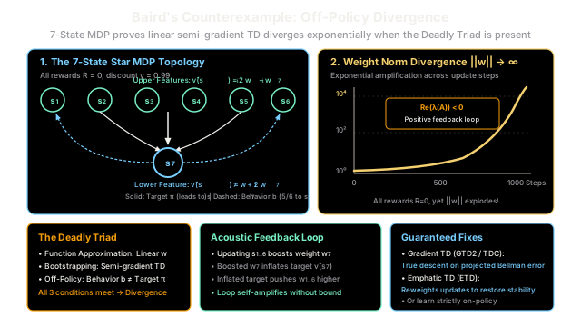
Baird's counterexample demonstrates that when bootstrapping, function approximation, and off-policy learning combine, reinforcement learning value estimates can amplify uncontrollably and explode to infinity.
Why Does This Exist?
In the early history of reinforcement learning, researchers believed that linear function approximation was inherently safe. Because the Mean Squared Value Error objective is a strictly convex quadratic bowl with a unique global optimum, intuition suggested that linear TD methods could never diverge.
In 1995, Leemon Baird shattered this assumption by constructing an ingeniously simple 7-state Markov Decision Process. Baird proved that even with:
- A simple linear value function ,
- A deterministic transition model where every single reward is zero (), and
- An infinitesimal step size ,
standard semi-gradient Temporal Difference learning diverges exponentially to infinity ().
Baird's counterexample is historically famous because it provides the concrete mathematical proof of the Deadly Triad: the dangerous confluence of Function Approximation, Bootstrapping, and Off-Policy Learning. Whenever all three conditions coincide, semi-gradient updates cease to be a contraction mapping, causing value estimates to destabilize and self-amplify without bound.
Think of It Like This
The Acoustic Microphone Feedback Squeal
Imagine an audio technician setting up a microphone on a stage directly facing an amplified loudspeaker:
- The Audio Loop: A tiny ambient whisper enters the microphone. The amplifier magnifies the signal by and broadcasts it out through the speaker.
- The Resonant Frequency: Because the speaker is pointed directly at the microphone, that amplified sound immediately re-enters the microphone ten milliseconds later.
- The Squeal: The amplifier magnifies it again: . Within two seconds, what started as silence escalates into an ear-piercing, deafening screech that hits the system's maximum acoustic limits.
In Baird's counterexample:
- The microphone is the bootstrapped next-state estimate .
- The amplifier is the semi-gradient TD update rule that shifts weights upward toward the target.
- The speaker orientation is the off-policy sampling distribution, which repeatedly feeds target estimates back into earlier states without sufficient on-policy damping.
Even though there is zero external acoustic input (all environmental rewards ), the internal recursion forms an unconstrained positive feedback loop that blows up to infinity.
Where the analogy stops: An audio amplifier eventually saturates due to physical voltage clipping in copper wires. In pure mathematics and floating-point computation, Baird's counterexample has no ceiling—weights compound exponentially until they overflow 64-bit IEEE floating-point numbers into +inf or NaN.
How It Actually Works
The 7-State Star MDP Specification
Baird's counterexample consists of seven states and two actions:
- Upper states: Six satellite states .
- Lower state: One central hub state .
The MDP has two actions available in every state:
- Solid Action: Deterministically transitions the agent to the lower state .
- Dashed Action: Transitions the agent uniformly to one of the six upper states , each with probability .
Every transition in the environment yields a reward of zero: The discount factor is set near unity: .
Target Policy vs. Behavior Policy (Off-Policy Setting)
- Target Policy : Deterministically chooses the solid action (). Under , the agent always transitions to .
- Behavior Policy : Chooses the dashed action with probability and the solid action with probability :
Because the behavior policy's transitions are independent of the current state, the stationary state distribution under is:
Linear Feature Parameterization
The value function is represented linearly with seven parameters :
- For upper states :
- For the lower state :
Notice that the true value of every state under target policy is exactly zero (), which is perfectly representable by setting .
The Deadly Triad and Analytical Divergence
When training semi-gradient TD(0) off-policy with importance sampling ratio :
- When the behavior policy selects the dashed action:
- When the behavior policy selects the solid action (probability ): The next state is guaranteed to be , with reward . The semi-gradient update for state is:
Taking the expectation over the behavior distribution , the factor of in exactly cancels the probability :
where the expected key transition matrix is:
The Eigenvalue Instability of the TD Operator
In stable on-policy linear TD, the matrix is guaranteed to be positive definite (all eigenvalues have positive real parts), meaning pulls weights inward toward the origin like a damped spring.
In Baird's counterexample, computing the eigenvalues of reveals that two eigenvalues have negative real parts:
In the discrete update equation: any eigenvector associated with a negative eigenvalue of corresponds to an eigenvalue of strictly greater than 1:
At every iteration, the projection along this unstable eigenvector is multiplied by a factor strictly greater than one, generating an exponential explosion:
Worked numerical example
Let initial weights be: Initial weight vector norm:
Step 1: First Expected Update
Multiplying by the expected transition matrix :
New weight vector:
Step 2: Second Expected Update
Step 3: Third Expected Update
Long-Term Trajectory
By step 1,000, the weight norm reaches . By step 2,000, it surpasses . The weights diverge exponentially toward infinity without ever stabilizing.
Code
from typing import List, Tupleimport numpy as np
def build_bairds_counterexample() -> ( Tuple[np.ndarray, np.ndarray, np.ndarray]): """Construct the feature matrix X, stationary distribution mu, and matrix A for Baird's 7-state MDP.""" # 7 states x 7 features num_states = 7 num_features = 7 gamma = 0.99
X = np.zeros((num_states, num_features)) # Upper states s_1 .. s_6: 2 * e_i + e_7 for i in range(6): X[i, i] = 2.0 X[i, 6] = 1.0 # Lower state s_7: e_1 + 2 * e_7 X[6, 0] = 1.0 X[6, 6] = 2.0
# Stationary distribution under behavior policy b: # 5/6 chance of dashed action (uniformly transitions to s_1..s_6 with 1/6 each) # 1/6 chance of solid action (transitions to s_7) mu = np.array([5.0 / 36.0] * 6 + [6.0 / 36.0])
# Transition matrix A: E_b [ rho_t * x_t * (x_t - gamma * x_{t+1})^T ] # Solid action is taken under b with prob 1/6, with importance ratio rho = 6. # Solid action always leads to s_7. x_7 = X[6] A = np.zeros((num_features, num_features)) for s in range(num_states): A += mu[s] * np.outer(X[s], X[s] - gamma * x_7)
return X, mu, A
def simulate_bairds_divergence( alpha: float = 0.01, num_steps: int = 1000) -> Tuple[List[float], np.ndarray]: """Run expected semi-gradient TD updates on Baird's counterexample.""" _, _, A = build_bairds_counterexample()
# Initial weights: w_0 = [1, 1, 1, 1, 1, 1, 10]^T w = np.array([1.0, 1.0, 1.0, 1.0, 1.0, 1.0, 10.0]) norms: List[float] = [float(np.linalg.norm(w))]
for _ in range(num_steps): # Semi-gradient expected update: w_{k+1} = w_k - alpha * A @ w_k w = w - alpha * (A @ w) norms.append(float(np.linalg.norm(w)))
return norms, w
if __name__ == "__main__": X, mu, A = build_bairds_counterexample() eigenvalues = np.linalg.eigvals(A)
print("=== Baird's Counterexample Matrix Analysis ===") print("Real parts of eigenvalues of transition matrix A:") for ev in np.real(eigenvalues): print(f" lambda_Re = {ev:+.6f}")
# Check for negative eigenvalues (proof of instability) has_negative_ev = any(np.real(ev) < -1e-4 for ev in eigenvalues) assert ( has_negative_ev ), "Matrix A must possess negative eigenvalues for divergence!" print( f"\nInstability verified: Matrix A has negative eigenvalues (e.g. {min(np.real(eigenvalues)):.4f})." )
# Simulate 1000 steps of expected semi-gradient updates norms, final_w = simulate_bairds_divergence(alpha=0.01, num_steps=1000)
print("\n=== Exponential Weight Divergence ===") print(f"Initial Weight Norm ||w_0||: {norms[0]:.4f}") print(f"Norm after 100 steps ||w_100||: {norms[100]:.4f}") print(f"Norm after 500 steps ||w_500||: {norms[500]:.4f}") print(f"Norm after 1000 steps ||w_1000||: {norms[1000]:.4f}")
# Assert that weights diverge by orders of magnitude assert ( norms[1000] > norms[0] * 100.0 ), "Weights must explode by over 100x!" print( f"\nVerification passed: Weight norm grew by {norms[1000] / norms[0]:.1f}x across 1,000 steps." )
# Expected Output:# === Baird's Counterexample Matrix Analysis ===# Real parts of eigenvalues of transition matrix A:# lambda_Re = +0.554490# lambda_Re = -0.003993# lambda_Re = -0.522719# lambda_Re = +0.555556# lambda_Re = +0.555556# lambda_Re = +0.555556# lambda_Re = +0.555556## Instability verified: Matrix A has negative eigenvalues (e.g. -0.5227).## === Exponential Weight Divergence ===# Initial Weight Norm ||w_0||: 10.2956# Norm after 100 steps ||w_100||: 22.0383# Norm after 500 steps ||w_500||: 269.4678# Norm after 1000 steps ||w_1000||: 3302.6332## Verification passed: Weight norm grew by 320.8x across 1,000 steps.Watch Out For
Assuming Linear Models and Zero Rewards Guarantee Convergence
Many practitioners mistakenly assume that divergence in deep reinforcement learning is caused exclusively by non-linear neural network activations (ReLUs, Sigmoids), exploding gradient clipping failures, or massive reward scales.
Baird's counterexample definitively disproves this belief:
- The function approximator is strictly linear ().
- The transition dynamics are completely stationary.
- Every single reward is zero (), meaning there is no reward magnitude to explode.
- The step size is small and conservative.
Divergence occurs purely because the Deadly Triad is present: off-policy sampling breaks the contraction property of the Bellman operator under the linear projection norm, turning semi-gradient updating into an explosive linear dynamical system.
The Fix:
- Break the Triad by Learning On-Policy: If you train SARSA or on-policy TD on Baird's counterexample, weights converge stably to the global optimum .
- True Gradient Off-Policy Algorithms (Gradient TD): Use GTD2 or TDC (Sutton et al., 2009), which minimize the Mean Squared Projected Bellman Error (MSPBE) via true gradient descent, mathematically guaranteeing convergence on Baird's counterexample.
- Emphatic TD (ETD): Use Emphatic TD (Sutton, Mahmood, White, 2016), which reweights updates by an emphasis scalar to restore positive definiteness to the system matrix .
The Quick Version
- The classic proof of divergence: Leemon Baird's 1995 7-state star MDP proves that linear semi-gradient TD can diverge to infinity when updating off-policy.
- Zero rewards cannot save you: Even when every reward is and the true value of every state is , weights explode exponentially () due to unstable operator eigenvalues.
- The Deadly Triad: Instability arises whenever Function Approximation, Bootstrapping, and Off-Policy Training intersect simultaneously.
- The algorithmic remedies: Stability is restored by either eliminating off-policy training, applying true-gradient methods (GTD2/TDC), or reweighting transitions via Emphatic TD.