The Deadly Triad

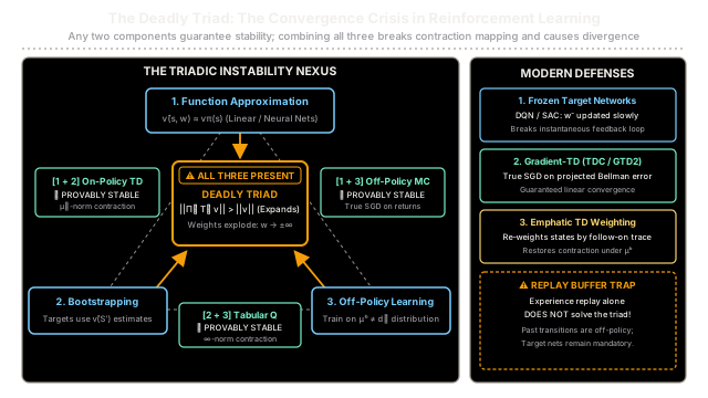
Combining function approximation, bootstrapping, and off-policy learning shatters the contraction mapping of the Bellman operator, causing unbounded value divergence.

Combining function approximation, bootstrapping, and off-policy learning breaks the contraction property of the projected Bellman operator, driving value estimates toward infinity.

Why Does This Exist?

In reinforcement learning, three architectural properties are universally desirable:

Function Approximation: The ability to scale to high-dimensional or continuous state spaces by representing value functions compactly with parameterized models $\hat{v}(s, \mathbf{w})$ (such as linear representations or deep neural networks) rather than lookup tables.
Bootstrapping: The ability to update value estimates from subsequent value estimates ( $R + \gamma \hat{v}(S')$ ) without waiting until the end of an episode, enabling online learning and massive reductions in sample variance.
Off-Policy Learning: The ability to evaluate or optimize a target policy $\pi$ while following a distinct behavior policy $b$ , enabling exploratory data collection, historical transition reuse, and parallel multi-task learning.

Individually, these three elements are the cornerstones of modern RL. Pairwise, any combination of two is provably stable and well-behaved.

However, Richard Sutton identified that combining all three simultaneously triggers a catastrophic phenomenon known as The Deadly Triad. When function approximation, bootstrapping, and off-policy learning collide, the projected Bellman operator loses its fundamental contraction mapping property. Instead of pulling value predictions toward a fixed point, updates expand errors iteratively, driving weights toward $\pm\infty$ and causing algorithms to diverge entirely.

Understanding the deadly triad explains why naive deep Q-learning fails without defensive stabilization tricks, why experience replay buffers can inadvertently worsen instability, and why specialized off-policy methods—such as Gradient-TD, Emphatic-TD, and frozen target networks—are necessary.

Think of It Like This

The Resonating Three-Legged Stool

Imagine an engineered three-legged stool where each individual leg is forged from heavy titanium:

Leg 1 (Generalization): Distributes weight across broad load-bearing surfaces rather than resting on isolated points.
Leg 2 (Self-Support): Braces its own frame by transferring stresses forward into adjacent struts.
Leg 3 (Independent Grounding): Rests securely on uneven or externally shifting terrain.

Any two legs paired together create a mechanically stable structure:

Legs 1 + 2 (On-policy TD): A solid bipod leaning against a wall; load pressures contract into the ground.
Legs 1 + 3 (Off-policy MC): A rigid brace resting on uneven terrain; forces dissipate through direct physical contact.
Legs 2 + 3 (Tabular Q-learning): A standard self-bracing frame anchored on discrete, non-overlapping floor tiles; vibrations cannot jump between tiles.

However, when all three legs are assembled together and subjected to dynamic loads, a catastrophic resonance frequency occurs. Because Leg 1 spreads errors across states, Leg 2 feeds those uncorrected estimates forward into future targets, and Leg 3 samples transitions that do not match the system's natural damping equilibrium, the forces form an acoustic feedback loop.

A slight shudder in Leg 1 amplifies the strain on Leg 2, which ricochets back through Leg 3 at twice the amplitude. Within seconds, the uncontrolled harmonic resonance tears the joints apart, violently shattering the stool under its own internal stress.

Where the analogy stops: In mechanical structures, harmonic resonance eventually dissipates once the materials fracture. In reinforcement learning algorithms, the program continues executing gradient updates indefinitely, driving weights to floating-point overflows (NaN or inf) unless defensive architectural constraints break the feedback loop.

How It Actually Works

The Mathematical Mechanism: Loss of Contraction Mapping

To understand why the triad causes divergence, consider the Bellman evaluation operator $T^\pi$ defined over state-value functions:

$(T^\pi v)(s) \doteq \sum_a \pi(a \mid s) \sum_{s', r} p(s', r \mid s, a) \left[ r + \gamma v(s') \right]$

In tabular reinforcement learning, $T^\pi$ is a $\gamma$ -contraction in the supremum norm ( $\| \cdot \|_\infty$ ):

$\| T^\pi v - T^\pi u \|_\infty \le \gamma \| v - u \|_\infty, \quad \forall v, u \in \mathbb{R}^{|\mathcal{S}|}$

Because $\gamma < 1$ , Banach's Fixed Point Theorem guarantees that repeatedly applying $T^\pi$ converges to the unique true value function $v_\pi$ .

When we introduce linear function approximation, the value function is constrained to the subspace spanned by feature vectors: $\mathcal{V}_{\mathbf{w}} = \{ \mathbf{\Phi}\mathbf{w} \mid \mathbf{w} \in \mathbb{R}^d \}$ , where $d \ll |\mathcal{S}|$ . Applying $T^\pi$ to an approximated value $\mathbf{\Phi}\mathbf{w}$ generally yields a function that falls outside $\mathcal{V}_{\mathbf{w}}$ . The update must project that result back onto $\mathcal{V}_{\mathbf{w}}$ using a projection operator $\Pi_\mu$ , weighted by the state distribution $\mu$ :

$\Pi_\mu v \doteq \arg\min_{\hat{v} \in \mathcal{V}_{\mathbf{w}}} \| v - \hat{v} \|_\mu^2$

The effective operator governing semi-gradient TD methods is the projected Bellman operator:

$\bar{T}^\pi \doteq \Pi_\mu T^\pi$

Why On-Policy Learning is Stable

When the agent samples transitions on-policy, $\mu = d_\pi$ (the stationary distribution under policy $\pi$ ). Two critical mathematical conditions hold:

The projection operator $\Pi_{d_\pi}$ is an orthogonal projection, meaning it is a non-expansion in the $d_\pi$ -norm: $\|\Pi_{d_\pi} v\|_{d_\pi} \le \|v\|_{d_\pi}$ .
The Bellman operator $T^\pi$ is a $\gamma$ -contraction in the $d_\pi$ -norm: $\|T^\pi v - T^\pi u\|_{d_\pi} \le \gamma \|v - u\|_{d_\pi}$ .

Because the composition of a non-expansion and a $\gamma$ -contraction is itself a $\gamma$ -contraction:

$\| \Pi_{d_\pi} T^\pi v - \Pi_{d_\pi} T^\pi u \|_{d_\pi} \le \|\Pi_{d_\pi}\|_{d_\pi} \|T^\pi v - T^\pi u\|_{d_\pi} \le 1 \cdot \gamma \|v - u\|_{d_\pi} = \gamma \|v - u\|_{d_\pi}$

By the Tsitsiklis and Van Roy (1996) theorem, on-policy linear TD(0) converges with probability 1 to a unique fixed point $\mathbf{w}^*$ satisfying:

$\| \mathbf{\Phi}\mathbf{w}^* - v_\pi \|_{d_\pi} \le \frac{1}{\sqrt{1 - \gamma^2}} \min_{\mathbf{w}} \| \mathbf{\Phi}\mathbf{w} - v_\pi \|_{d_\pi}$

Why Off-Policy Learning Breaks the Contraction

When the agent collects data under a behavior policy $b \neq \pi$ , the data distribution is $\mu_b$ . Crucially, the target Bellman operator $T^\pi$ is not a contraction with respect to the behavior norm $\|\cdot\|_{\mu_b}$ .

While $\Pi_{\mu_b}$ remains a non-expansion in the $\mu_b$ -norm, $T^\pi$ can expand distances in that norm:

$\| T^\pi v - T^\pi u \|_{\mu_b} > \| v - u \|_{\mu_b}$

As a result, the spectral radius of the composite operator can exceed 1:

$\rho(\Pi_{\mu_b} T^\pi) > 1$

Iterating this operator repeatedly amplifies approximation errors rather than shrinking them. The parameters $\mathbf{w}_t$ grow exponentially, causing catastrophic value divergence.

The Three Pairwise Stable Regimes

Configuration	What Is Active	What Is Excluded	Stability Guarantee	Core Example
Approximation + Bootstrapping	Linear/NN models, TD targets	Off-policy (uses on-policy data $\mu = d_\pi$ )	Provably Stable: Contraction in $d_\pi$ -norm (Tsitsiklis & Van Roy)	On-Policy Linear TD, SARSA
Approximation + Off-Policy	Linear/NN models, Behavior $b \neq \pi$	Bootstrapping (uses full returns $G_t$ )	Provably Stable: True SGD on Mean Squared Value Error ( $\overline{\text{VE}}$ )	Gradient Monte Carlo, Off-Policy MC
Bootstrapping + Off-Policy	TD targets, Behavior $b \neq \pi$	Function Approximation (lookup table)	Provably Stable: Contraction in supremum norm ( $\\|\cdot\\|_\infty$ )	Tabular Q-Learning, Watkin's Q
The Deadly Triad	Approx + Bootstrap + Off-Policy	None	DIVERGENT: Projected Bellman operator expands errors	Off-policy linear TD, Baird's Counterexample

Worked Numerical Example: The Minimal 2-State Divergence

Consider the classic two-state counterexample formulated by Tsitsiklis & Van Roy (1996) and Sutton & Barto:

Two states: $\mathcal{S} = \{1, 2\}$ .
Single scalar parameter: $w \in \mathbb{R}$ ( $d = 1$ ).
Linear feature representations:
- State 1: $x(1) = 1.0 \implies \hat{v}(1, w) = 1.0 \cdot w$
- State 2: $x(2) = 2.0 \implies \hat{v}(2, w) = 2.0 \cdot w$
Transition dynamics under target policy $\pi$ $π$ :
- State 1 always transitions to State 2 with reward $R = 0$ .
- State 2 always transitions to State 2 with reward $R = 0$ .
Hyperparameters:
- Discount factor: $\gamma = 0.9$
- Learning rate: $\alpha = 0.1$
- Initial weight: $w_0 = 10.0$

1. The Deadly Triad Active (Divergence)

Under the behavior policy $b$ , the agent only observes transitions starting from State 1 ( $\mu_b(1) = 1.0, \mu_b(2) = 0.0$ ): Transition sampled: $(S = 1, R = 0, S' = 2)$ .

On step $k$ , the semi-gradient TD(0) update is:

Target: $U_k = R + \gamma \hat{v}(2, w_k) = 0 + 0.9 \times (2.0 \cdot w_k) = 1.8 \cdot w_k$
Current estimate: $\hat{v}(1, w_k) = 1.0 \cdot w_k$
TD Error: $\delta_k = U_k - \hat{v}(1, w_k) = 1.8 w_k - 1.0 w_k = 0.8 \cdot w_k$
Weight update: $w_{k+1} = w_k + \alpha \delta_k \nabla \hat{v}(1, w_k) = w_k + 0.1 \times (0.8 w_k) \times 1.0 = w_k (1 + 0.08) = 1.08 \cdot w_k$

Because the multiplier $1.08 > 1$ , the weights grow geometrically:

Step 0: $w_0 = 10.0000$
Step 1: $w_1 = 10.0000 \times 1.08 = 10.8000$
Step 2: $w_2 = 10.8000 \times 1.08 = 11.6640$
Step 3: $w_3 = 11.6640 \times 1.08 = 12.5971$
Step 4: $w_4 = 12.5971 \times 1.08 = 13.6049$
Step 5: $w_5 = 13.6049 \times 1.08 = 14.6933$
Step 10: $w_{10} = 10.0 \times (1.08)^{10} = 21.5892 \to \infty$

The value estimates explode without bound.

2. Disabling Bootstrapping (Monte Carlo / Pairwise Stable)

Replace the bootstrap estimate with the true episodic return. Because all transitions yield $R = 0$ , the full empirical return from State 1 is always $G = 0$ :

Target: $G = 0.0$
Current estimate: $\hat{v}(1, w_k) = 1.0 \cdot w_k$
Error: $\delta_k = 0.0 - w_k = -w_k$
Update: $w_{k+1} = w_k + \alpha (-w_k)(1.0) = w_k (1 - 0.1) = 0.9 \cdot w_k$

The multiplier is $0.9 < 1$ . The weights contract stably toward the true value $w^* = 0$ :

$w_0 = 10.0000 \to w_1 = 9.0000 \to w_2 = 8.1000 \to w_5 = 5.9049 \to 0$ .

3. Disabling Off-Policy Sampling (On-Policy / Pairwise Stable)

Under the target policy, suppose the agent follows a recurrent cycle $1 \to 2 \to 1$ with balanced stationary visitation $\mu(1) = 0.5, \mu(2) = 0.5$ :

From State 1 ( $1 \to 2, R = 0$ ): $\delta_1 = 0.9(2w) - 1w = +0.8w$ , gradient $x(1) = 1.0$ .
From State 2 ( $2 \to 1, R = 0$ ): $\delta_2 = 0.9(1w) - 2w = -1.1w$ , gradient $x(2) = 2.0$ .
Expected update: $\mathbb{E}[\Delta w] = 0.5 \alpha [\delta_1 x(1) + \delta_2 x(2)] = 0.5 (0.1) [0.8w(1.0) + (-1.1w)(2.0)] = 0.05 [0.8w - 2.2w] = -0.07 w$ $w_{k+1} = w_k (1 - 0.07) = 0.93 \cdot w_k$

The multiplier is $0.93 < 1$ . On-policy distribution weighting forces the updates to contract stably toward $w^* = 0$ .

Code

1from typing import Dict, List, Tuple2
3
4class DeadlyTriadComparison:5    """Demonstrates how the deadly triad triggers divergence and how6
7    removing any single component restores mathematical stability.8    """9
10    def __init__(self, gamma: float = 0.9, alpha: float = 0.1, w0: float = 10.0) -> None:11        self.gamma = gamma12        self.alpha = alpha13        self.w0 = w014
15    def run_deadly_triad(self, steps: int = 10) -> List[float]:16        """Triad active: Linear approx [v(1)=w, v(2)=2w], Bootstrapping [target=gamma*v(2)],17
18        Off-policy [only sampling state 1 -> 2].19        """20        w = self.w021        trajectory = [w]22        for _ in range(steps):23            target = self.gamma * (2.0 * w)  # R=0 + gamma * v_hat(2, w)24            prediction = 1.0 * w             # v_hat(1, w)25            error = target - prediction       # (2*gamma - 1) * w = +0.8 w26            gradient = 1.027            w += self.alpha * error * gradient28            trajectory.append(w)29        return trajectory30
31    def run_without_bootstrapping(self, steps: int = 10) -> List[float]:32        """Pairwise Stable: Function approx + Off-policy, but NO bootstrapping33
34        (Monte Carlo target G = 0).35        """36        w = self.w037        trajectory = [w]38        for _ in range(steps):39            target = 0.0                     # Unbiased return G_t = 040            prediction = 1.0 * w41            error = target - prediction42            gradient = 1.043            w += self.alpha * error * gradient44            trajectory.append(w)45        return trajectory46
47    def run_without_off_policy(self, steps: int = 10) -> List[float]:48        """Pairwise Stable: Function approx + Bootstrapping, but ON-POLICY data49
50        (balanced transitions 1 -> 2 and 2 -> 1).51        """52        w = self.w053        trajectory = [w]54        for _ in range(steps):55            # Transition 1 -> 2 (visited 50% of the time)56            t1 = self.gamma * (2.0 * w)57            p1 = 1.0 * w58            d1 = t1 - p159            g1 = 1.060
61            # Transition 2 -> 1 (visited 50% of the time)62            t2 = self.gamma * (1.0 * w)63            p2 = 2.0 * w64            d2 = t2 - p265            g2 = 2.066
67            # Average on-policy expectation68            expected_delta_w = 0.5 * (d1 * g1 + d2 * g2)69            w += self.alpha * expected_delta_w70            trajectory.append(w)71        return trajectory72
73    def run_without_approximation(self, steps: int = 10) -> List[Tuple[float, float]]:74        """Pairwise Stable: Bootstrapping + Off-policy, but TABULAR representation75
76        (lookup table with separate V[1] and V[2]).77        """78        v: Dict[int, float] = {1: self.w0, 2: 2.0 * self.w0}79        trajectory = [(v[1], v[2])]80        for _ in range(steps):81            target = 0.0 + self.gamma * v[2]82            error = target - v[1]83            v[1] += self.alpha * error84            trajectory.append((v[1], v[2]))85        return trajectory86
87
88if __name__ == "__main__":89    sim = DeadlyTriadComparison(gamma=0.9, alpha=0.1, w0=10.0)90
91    divergent = sim.run_deadly_triad(steps=5)92    mc_stable = sim.run_without_bootstrapping(steps=5)93    on_policy_stable = sim.run_without_off_policy(steps=5)94    tabular_stable = sim.run_without_approximation(steps=5)95
96    print("Step | Triad (Diverges) | No Bootstrap (MC) | On-Policy (TD) | Tabular V[1]")97    print("-" * 72)98    for step in range(6):99        print(100            f"{step:4d} | "101            f"{divergent[step]:16.4f} | "102            f"{mc_stable[step]:17.4f} | "103            f"{on_policy_stable[step]:14.4f} | "104            f"{tabular_stable[step][0]:13.4f}"105        )

1# Expected Output:2# Step | Triad (Diverges) | No Bootstrap (MC) | On-Policy (TD) | Tabular V[1]3# ------------------------------------------------------------------------4#    0 |          10.0000 |           10.0000 |        10.0000 |       10.00005#    1 |          10.8000 |            9.0000 |         9.3000 |       10.80006#    2 |          11.6640 |            8.1000 |         8.6490 |       11.52007#    3 |          12.5971 |            7.2900 |         8.0436 |       12.16808#    4 |          13.6049 |            6.5610 |         7.4805 |       12.75129#    5 |          14.6933 |            5.9049 |         6.9569 |       13.2761

Watch Out For

The Experience Replay Illusion

A common misconception among deep reinforcement learning practitioners is assuming that an Experience Replay Buffer eliminates the deadly triad by breaking temporal correlations between consecutive transitions.

In reality, experience replay amplifies the off-policy condition. Transitions sampled from a replay buffer were generated by historical policy checkpoints ( $\pi_{\theta_{t-k}}$ ) that differ substantially from the currently active policy ( $\pi_{\theta_t}$ ). When combined with neural network function approximation and 1-step TD bootstrapping, an experience replay buffer satisfies every condition of the deadly triad.

If you train a deep Q-network using a replay buffer without frozen target networks, Q-values diverge rapidly, culminating in gradient explosion and policy collapse.

The Fix: Decouple the bootstrapping target from the online parameters. Use an explicitly frozen target network ( $\mathbf{w}^-$ ) whose parameters are only periodically synchronized or softly tracked via Polyak averaging:

$\mathbf{w}^- \leftarrow \tau \mathbf{w} + (1 - \tau) \mathbf{w}^-, \quad \tau \ll 1$

Target: $Y_t = R_{t+1} + \gamma \max_{a'} Q(S_{t+1}, a'; \mathbf{w}^-)$ . Because $\mathbf{w}^-$ is quasi-static relative to the fast inner-loop gradient updates on $\mathbf{w}$ , it breaks the instantaneous self-reinforcing feedback loop. Alternatively, use provably convergent off-policy algorithms such as TDC (Two Time-Scale Gradient-TD) or Emphatic-TD.

The Quick Version

Three Essential Ingredients: Function approximation, bootstrapping, and off-policy learning are all required to trigger the deadly triad; removing any single component restores mathematical convergence guarantees.
Contraction Mapping Loss: Off-policy sampling disrupts the stationary distribution weighting, allowing the projected Bellman operator $\Pi_{\mu_b} T^\pi$ to expand errors ( $\|\Pi_{\mu_b} T^\pi\| > 1$ ) rather than contract them.
Geometric Value Explosion: Even in simple 2-state environments with zero rewards, unmitigated updates multiply weights by $(1 + \alpha(2\gamma - 1)) > 1$ each step, driving predictions toward $\pm\infty$ .
Modern Mitigations: Deep RL controls the triad using frozen target networks ( $\mathbf{w}^-$ ) and Polyak averaging, while theoretical RL uses Gradient-TD (GTD2/TDC) and Emphatic-TD to restore contraction.