Off-Policy Learning with Approximation

Combining off-policy data, bootstrapping, and function approximation creates the Deadly Triad, where Bellman targets expand rather than contract, driving value estimates toward infinity.

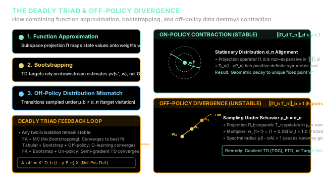
Off-policy learning with function approximation breaks the contraction property of the projected Bellman operator, causing unbounded parameter divergence.

Why Does This Exist?

Modern reinforcement learning systems must satisfy three practical requirements simultaneously:

Generalization across massive state spaces: Tabular lookups cannot represent continuous control or high-dimensional sensory inputs like images, requiring parametric function approximation $\hat{v}(s, \mathbf{w}) \approx v_\pi(s)$ .
Sample efficiency through online updating: Waiting for entire trajectories to complete (Monte Carlo rollouts) is high-variance and impossible in non-terminating tasks, requiring 1-step temporal difference bootstrapping $R_{t+1} + \gamma \hat{v}(S_{t+1}, \mathbf{w})$ .
Exploration and sample reuse: Agents must explore safely while evaluating greedy target policies, reuse historical transition transitions from replay buffers, or evaluate multiple parallel behaviors from a single stream of experience, requiring off-policy data where the behavior distribution $\mu_b$ differs from the target stationary distribution $d_\pi$ .

When used separately or in pairs, reinforcement learning algorithms remain provably stable:

Tabular + Bootstrapping + Off-Policy: Standard tabular Q-learning converges to $q^*$ with probability 1 because the tabular Bellman operator is an infinity-norm contraction ( $\|T \mathbf{q}_1 - T \mathbf{q}_2\|_\infty \le \gamma \|\mathbf{q}_1 - \mathbf{q}_2\|_\infty$ ).
Function Approximation + Off-Policy (No Bootstrapping): Monte Carlo policy evaluation with linear features is standard supervised regression. It minimizes mean-squared error with no feedback loop, guaranteeing stable convergence to the minimum-error projection.
Function Approximation + Bootstrapping + On-Policy: Semi-gradient $\text{TD}(0)$ contracts under the stationary distribution weighted norm $\|\cdot\|_{d_\pi}$ , converging to a unique fixed point $\mathbf{w}^*$ .

However, combining all three elements forms what Richard Sutton termed The Deadly Triad. When bootstrapping targets are projected onto a lower-dimensional feature subspace under an off-policy visitation distribution $\mu_b$ , the composite projected Bellman operator $\Pi_b T_\pi$ ceases to be a contraction mapping. The update matrix develops eigenvalues with negative real parts, turning stable temporal difference corrections into an explosive positive feedback loop where weights grow exponentially toward infinity.

Think of It Like This

The Outdated Map and the Echoing Detour

Imagine an automated highway logistics planner trying to estimate driving times between cities. The planner uses a compressed lookup table that groups adjacent towns into single generalized regions (function approximation).

To update transit estimates without waiting for trucks to complete thousand-mile hauls, the dispatcher updates the departure city's estimate using the current estimate of the next town along the route plus the immediate leg's toll-booth time (bootstrapping).

However, the fleet is currently routed through rural secondary detours due to winter storms, so real trucks only visit rural backroads rather than the main interstates (off-policy sampling). When a driver on a detour reports a slight delay, the regional lookup table inadvertently raises the estimated transit time for both the rural road and the adjacent highway interchange.

On the next iteration, the bootstrapped calculation treats this newly inflated interchange estimate as ground truth. Because actual trucks rarely traverse the primary highway under the storm routing, the algorithm never gathers empirical evidence to correct the inflation. Instead, the inflated highway value feeds back into the rural detour calculation, which inflates the interchange further, echoing endlessly until the software predicts a 5-minute commute will take 10 million hours.

Where the analogy stops: Real-world fleet dispatchers can compare route plans against absolute GPS timestamps to reset drift. In semi-gradient temporal difference learning, there is no global supervising timestamp—the algorithm blindly trusts its own parameterized predictions as targets, creating runaway divergence when distribution weighting does not align with transition dynamics.

How It Actually Works

The Deadly Triad and Projected Bellman Divergence

Consider linear function approximation where the value of state $s$ is approximated as:

$\hat{v}(s, \mathbf{w}) = \mathbf{w}^\top \mathbf{x}(s)$

where $\mathbf{x}(s) \in \mathbb{R}^d$ is the feature vector of state $s$ and $\mathbf{w} \in \mathbb{R}^d$ is the parameter vector. In matrix notation across all states $\mathcal{S} = \{s_1, \dots, s_n\}$ , $\mathbf{v} = \mathbf{X}\mathbf{w}$ , where $\mathbf{X} \in \mathbb{R}^{n \times d}$ is the feature matrix.

Let $\mathbf{D}_b = \text{diag}(\mu_b(s_1), \dots, \mu_b(s_n))$ be the diagonal matrix of state visitation probabilities under the behavior policy $b$ . The weighted least-squares projection operator $\Pi_b$ maps any arbitrary state-value vector $\mathbf{v} \in \mathbb{R}^n$ onto the linear subspace spanned by $\mathbf{X}$ :

$\Pi_b = \mathbf{X} (\mathbf{X}^\top \mathbf{D}_b \mathbf{X})^{-1} \mathbf{X}^\top \mathbf{D}_b$

The target policy Bellman evaluation operator $T_\pi$ maps value vectors via:

$T_\pi \mathbf{v} = \mathbf{r}_\pi + \gamma \mathbf{P}_\pi \mathbf{v}$

where $\mathbf{r}_\pi(s) = \sum_a \pi(a|s) \mathcal{R}(s, a)$ is the expected reward vector, $\mathbf{P}_\pi(s, s') = \sum_a \pi(a|s) \mathcal{P}(s'|s, a)$ is the state transition probability matrix, and $\gamma \in [0, 1)$ is the discount factor.

Semi-gradient linear TD seeks a parameter vector $\mathbf{w}$ satisfying the projected Bellman equation:

$\mathbf{X}\mathbf{w} = \Pi_b T_\pi (\mathbf{X}\mathbf{w}) = \Pi_b (\mathbf{r}_\pi + \gamma \mathbf{P}_\pi \mathbf{X}\mathbf{w})$

Multiplying both sides by $\mathbf{X}^\top \mathbf{D}_b$ removes the projection inversion $(\mathbf{X}^\top \mathbf{D}_b \mathbf{X})^{-1}$ , yielding the linear system:

$\mathbf{X}^\top \mathbf{D}_b \mathbf{X}\mathbf{w} = \mathbf{X}^\top \mathbf{D}_b (\mathbf{r}_\pi + \gamma \mathbf{P}_\pi \mathbf{X}\mathbf{w})$

Rearranging into standard form $\mathbf{A}\mathbf{w} = \mathbf{b}$ :

$\mathbf{A} = \mathbf{X}^\top \mathbf{D}_b (\mathbf{I} - \gamma \mathbf{P}_\pi) \mathbf{X}$

$\mathbf{b} = \mathbf{X}^\top \mathbf{D}_b \mathbf{r}_\pi$

The expected continuous parameter evolution under semi-gradient TD updates with step size $\alpha_t$ follows the ordinary differential equation (ODE):

$\mathbb{E}[\Delta \mathbf{w}_t] = \alpha_t (\mathbf{b} - \mathbf{A}\mathbf{w}_t)$

For the discrete iteration $\mathbf{w}_{t+1} = \mathbf{w}_t + \alpha (\mathbf{b} - \mathbf{A}\mathbf{w}_t) = (\mathbf{I} - \alpha \mathbf{A})\mathbf{w}_t + \alpha \mathbf{b}$ to converge to $\mathbf{w}^* = \mathbf{A}^{-1}\mathbf{b}$ , the matrix $\mathbf{A}$ must be positive definite (all eigenvalues of $\mathbf{A}$ must have strictly positive real parts, $\text{Re}(\lambda_i) > 0$ ).

On-Policy Stability ( $\mathbf{D}_b = \mathbf{D}_\pi$ ): When transitions are sampled from the target policy's stationary distribution $d_\pi$ , the matrix $\mathbf{D}_\pi (\mathbf{I} - \gamma \mathbf{P}_\pi)$ has a strictly positive-definite symmetric part:

$\mathbf{y}^\top \mathbf{D}_\pi (\mathbf{I} - \gamma \mathbf{P}_\pi) \mathbf{y} > 0 \quad \forall \mathbf{y} \neq \mathbf{0}$

Because $\mathbf{X}$ has full column rank, $\mathbf{A} = \mathbf{X}^\top \mathbf{D}_\pi (\mathbf{I} - \gamma \mathbf{P}_\pi) \mathbf{X}$ is positive definite. The composite operator $\Pi_\pi T_\pi$ is a contraction with modulus $\gamma$ in the $\|\cdot\|_{d_\pi}$ norm, guaranteeing convergence to a unique solution with bounded approximation error:

$\|v_{\mathbf{w}^*} - v_\pi\|_{d_\pi} \le \frac{1}{\sqrt{1 - \gamma^2}} \|\Pi_\pi v_\pi - v_\pi\|_{d_\pi}$
Off-Policy Instability ( $\mathbf{D}_b \neq \mathbf{D}_\pi$ ): When data arrives from behavior distribution $\mu_b$ , the weighting matrix $\mathbf{D}_b$ does not balance the target transition matrix $\mathbf{P}_\pi$ . The symmetric part $\frac{1}{2}(\mathbf{A} + \mathbf{A}^\top)$ can have negative eigenvalues.

When $\mathbf{A}$ has an eigenvalue $\lambda$ with $\text{Re}(\lambda) < 0$ , the transition matrix $(\mathbf{I} - \alpha \mathbf{A})$ has an eigenvalue with magnitude $|1 - \alpha \lambda| > 1$ . The spectral radius satisfies $\rho(\mathbf{I} - \alpha \mathbf{A}) > 1$ , causing $\|\mathbf{w}_t\| \to \infty$ at a geometric rate regardless of step size magnitude.

Worked numerical example

To observe divergence directly, consider the classic minimal counterexample introduced by John Tsitsiklis and Benjamin Van Roy (1997):

Environment: Two states $\mathcal{S} = \{s_1, s_2\}$ .
Feature Representation: A single parameter $w \in \mathbb{R}$ ( $d = 1$ ): $\mathbf{x}(s_1) = 1.0, \quad \mathbf{x}(s_2) = 2.0$ Approximated values: $\hat{v}(s_1, w) = 1.0 \cdot w$ , $\hat{v}(s_2, w) = 2.0 \cdot w$ .
Target Policy $\pi$ : Moves deterministically from $s_1 \to s_2$ with reward $R = 0$ , and remains in $s_2 \to s_2$ with reward $R = 0$ .
Discount Factor: $\gamma = 0.9$ .
True Values: Because all rewards are zero, $v_\pi(s_1) = 0$ and $v_\pi(s_2) = 0$ . The optimal parameter is $w^* = 0$ .
Learning Rate: $\alpha = 0.1$ . Initial parameter: $w_0 = 10.0$ .

Scenario A: Off-Policy Sampling (Divergence)

Suppose the behavior policy $b$ samples only the transition $s_1 \to s_2$ with reward $R = 0$ (visitation $\mu_b(s_1) = 1.0, \mu_b(s_2) = 0.0$ ):

The temporal difference error at step $t$ is:

$\delta_t = R_{t+1} + \gamma \hat{v}(s_2, w_t) - \hat{v}(s_1, w_t) = 0 + 0.9 (2.0 w_t) - 1.0 w_t = (1.8 - 1.0) w_t = +0.8 w_t$

The semi-gradient linear TD update rule is:

$w_{t+1} = w_t + \alpha \delta_t \mathbf{x}(s_1) = w_t + 0.1 (+0.8 w_t)(1.0) = (1 + 0.08) w_t = 1.08 w_t$

Let's compute the parameter trajectory step by step:

Step 0: $w_0 = 10.0000$ $\delta_0 = 0.8 \times 10.0000 = +8.0000$
Step 1: $w_1 = 10.0000 + 0.1 \times 8.0000 \times 1.0 = 10.8000$ $\delta_1 = 0.8 \times 10.8000 = +8.6400$
Step 2: $w_2 = 10.8000 + 0.1 \times 8.6400 \times 1.0 = 11.6640$ $\delta_2 = 0.8 \times 11.6640 = +9.3312$
Step 3: $w_3 = 11.6640 + 0.1 \times 9.3312 \times 1.0 = 12.5971$

Because the multiplier $1.08 > 1.0$ , after $k$ steps $w_k = 10.0 \times (1.08)^k$ . As $k \to \infty$ , $w_k \to +\infty$ .

Scenario B: On-Policy Sampling (Convergence)

Now suppose data is sampled on-policy from the target policy's true stationary distribution. In policy $\pi$ , state $s_2$ is absorbing, so the stationary distribution is $d_\pi(s_1) = 0.0, d_\pi(s_2) = 1.0$ .

Transitions sampled in $s_2$ move $s_2 \to s_2$ with reward $R = 0$ :

$\delta_t = R_{t+1} + \gamma \hat{v}(s_2, w_t) - \hat{v}(s_2, w_t) = 0 + 0.9(2.0 w_t) - 2.0 w_t = (1.8 - 2.0) w_t = -0.2 w_t$

The semi-gradient linear TD update rule is:

$w_{t+1} = w_t + \alpha \delta_t \mathbf{x}(s_2) = w_t + 0.1 (-0.2 w_t)(2.0) = (1 - 0.04) w_t = 0.96 w_t$

Computing the on-policy trajectory:

Step 0: $w_0 = 10.0000$ $\delta_0 = -0.2 \times 10.0000 = -2.0000$
Step 1: $w_1 = 10.0000 + 0.1 \times (-2.0000) \times 2.0 = 9.6000$ $\delta_1 = -0.2 \times 9.6000 = -1.9200$
Step 2: $w_2 = 9.6000 + 0.1 \times (-1.9200) \times 2.0 = 9.2160$ $\delta_2 = -0.2 \times 9.2160 = -1.8432$
Step 3: $w_3 = 9.2160 + 0.1 \times (-1.8432) \times 2.0 = 8.8474$

Because the multiplier $0.96 < 1.0$ , the parameter contracts geometrically toward the true target value $w^* = 0.0$ .

Code

The following self-contained Python script simulates the Tsitsiklis & Van Roy two-state counterexample, contrasting off-policy divergence with on-policy contraction.

1from typing import List, Tuple2
3class TwoStateLinearTD:4    """Simulates linear semi-gradient TD on the Tsitsiklis & Van Roy counterexample."""5
6    def __init__(self, gamma: float = 0.9, alpha: float = 0.1) -> None:7        self.gamma: float = gamma8        self.alpha: float = alpha9        # State features: x(s1) = 1.0, x(s2) = 2.010        self.features: dict[str, float] = {"s1": 1.0, "s2": 2.0}11
12    def v_hat(self, state: str, w: float) -> float:13        """Evaluate linear value function approximation."""14        return w * self.features[state]15
16    def off_policy_step(self, w: float) -> Tuple[float, float]:17        """Perform one off-policy TD update on transition s1 -> s2 (reward = 0)."""18        reward = 0.019        td_target = reward + self.gamma * self.v_hat("s2", w)20        delta = td_target - self.v_hat("s1", w)21        w_next = w + self.alpha * delta * self.features["s1"]22        return delta, w_next23
24    def on_policy_step(self, w: float) -> Tuple[float, float]:25        """Perform one on-policy TD update on absorbing transition s2 -> s2 (reward = 0)."""26        reward = 0.027        td_target = reward + self.gamma * self.v_hat("s2", w)28        delta = td_target - self.v_hat("s2", w)29        w_next = w + self.alpha * delta * self.features["s2"]30        return delta, w_next31
32    def run_comparison(self, w_initial: float = 10.0, steps: int = 3) -> None:33        print(f"Initial weight: w0 = {w_initial:.4f}")34        print("=" * 60)35
36        # Off-policy simulation37        print("--- OFF-POLICY (Behavior samples s1 -> s2) ---")38        w_off = w_initial39        for step in range(1, steps + 1):40            delta, w_off = self.off_policy_step(w_off)41            print(f"Step {step}: delta = {delta:+.4f}, w_{step} = {w_off:.4f}")42
43        # On-policy simulation44        print("\n--- ON-POLICY (Stationary visitation s2 -> s2) ---")45        w_on = w_initial46        for step in range(1, steps + 1):47            delta, w_on = self.on_policy_step(w_on)48            print(f"Step {step}: delta = {delta:+.4f}, w_{step} = {w_on:.4f}")49
50        print("=" * 60)51        print(f"Final Off-Policy weight: {w_off:.4f} (EXPANDING)")52        print(f"Final On-Policy weight:  {w_on:.4f} (CONTRACTING)")53
54        # Invariants55        assert w_off > w_initial, "Off-policy weights must diverge"56        assert w_on < w_initial, "On-policy weights must contract"57
58if __name__ == "__main__":59    sim = TwoStateLinearTD(gamma=0.9, alpha=0.1)60    sim.run_comparison(w_initial=10.0, steps=3)

1# -> expected output:2Initial weight: w0 = 10.00003============================================================4--- OFF-POLICY (Behavior samples s1 -> s2) ---5Step 1: delta = +8.0000, w_1 = 10.80006Step 2: delta = +8.6400, w_2 = 11.66407Step 3: delta = +9.3312, w_3 = 12.59718
9--- ON-POLICY (Stationary visitation s2 -> s2) ---10Step 1: delta = -2.0000, w_1 = 9.600011Step 2: delta = -1.9200, w_2 = 9.216012Step 3: delta = -1.8432, w_3 = 8.847413============================================================14Final Off-Policy weight: 12.5971 (EXPANDING)15Final On-Policy weight:  8.8474 (CONTRACTING)

Watch Out For

The False Safety of Ordinary Importance Sampling

A common misconception is that weighting transitions with per-step importance sampling ratios $\rho_t = \frac{\pi(A_t|S_t)}{b(A_t|S_t)}$ stabilizes off-policy semi-gradient algorithms.

While per-step importance sampling reweights action probabilities to compute unbiased expectations over target actions $\pi(\cdot|S_t)$ , it does not alter the underlying state distribution $\mu_b$ . The sequence of states $S_t$ visited by the agent continues to follow the behavior policy's visitation frequency $\mu_b$ , not the target policy's stationary distribution $d_\pi$ .

Because the state weighting matrix remains $\mathbf{D}_b$ , the key matrix $\mathbf{A} = \mathbf{X}^\top \mathbf{D}_b (\mathbf{I} - \gamma \mathbf{P}_\pi) \mathbf{X}$ can still possess negative eigenvalues. Semi-gradient TD with ordinary importance sampling can diverge just as violently as unweighted TD, with the added drawback of extreme variance from the product of likelihood ratios.

The Fix: To achieve true stability under the Deadly Triad, practitioners must employ methods that fundamentally resolve the distribution mismatch:

True Gradient Methods (Gradient TD / TDC / GTD2): Minimize the Mean Squared Projected Bellman Error (MSPBE) via two-timescale stochastic gradient descent, ensuring convergence regardless of off-policy distributions.
Emphatic TD (ETD): Reweight state updates by tracking an emphasis scalar $M_t = \gamma \rho_{t-1} M_{t-1} + I_t$ that restores stationary distribution weighting in expectation.
Deep RL Stabilizers (DQN / SAC): Decouple bootstrap targets using slowly updating Polyak or periodic target networks ( $\mathbf{w}^-$ ) and reward clipping to limit feedback amplification within replay buffers.

The Quick Version

The Deadly Triad: Instability occurs exclusively when function approximation, bootstrapping, and off-policy data are combined simultaneously; removing any one guarantees convergence.
Lost Contraction: While on-policy projected Bellman operators contract with modulus $\gamma$ in the stationary norm $\|\cdot\|_{d_\pi}$ , off-policy operators $\Pi_b T_\pi$ expand distances under behavior weighting $\|\cdot\|_{\mu_b}$ .
Negative Eigenvalues: The expected update matrix $\mathbf{A} = \mathbf{X}^\top \mathbf{D}_b (\mathbf{I} - \gamma \mathbf{P}_\pi) \mathbf{X}$ is not positive definite when $\mathbf{D}_b \neq \mathbf{D}_\pi$ , producing spectral radius $\rho(\mathbf{I} - \alpha \mathbf{A}) > 1$ and unbounded parameter growth.
Importance Sampling Limitation: Per-step action importance sampling corrects action choice probabilities but fails to fix state visitation mismatch $\mu_b \neq d_\pi$ , requiring Gradient TD (TDC/GTD2) or target networks for stability.