Gradient-TD Methods (TDC & GTD2)
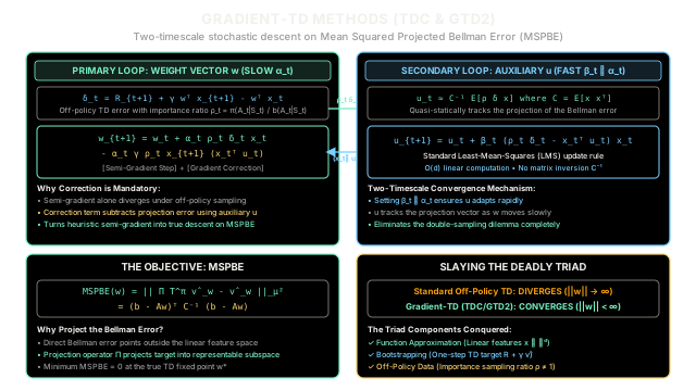
Standard TD methods can diverge when combining function approximation, bootstrapping, and off-policy sampling. Gradient-TD methods guarantee convergence by directly minimizing the projected Bellman error using a two-timescale weight update.
Why Does This Exist?
In reinforcement learning, the combination of three elements forms the notorious Deadly Triad:
- Function approximation (linear features or neural networks instead of tabular lookups)
- Bootstrapping (updating value estimates toward downstream value estimates rather than full Monte Carlo returns)
- Off-policy learning (evaluating or optimizing a target policy while observing transitions generated by an exploratory behavior policy )
When all three conditions hold simultaneously, standard semi-gradient Temporal Difference methods like TD(0) and Q-learning can diverge to infinity. Under an off-policy distribution , the transition operator is no longer a contraction mapping with respect to the state distribution weighting matrix . As a result, semi-gradient TD updates do not follow the true negative gradient of any objective function. The underlying expected update matrix can have eigenvalues with negative real parts, causing value weights to explode exponentially—as vividly demonstrated by Baird's counterexample.
Early attempts to fix this divergence attempted to minimize the Mean Squared Bellman Error (). However, the true gradient of contains a product of expectations, creating the notorious double-sampling problem: computing an unbiased sample gradient requires observing two independent next states from the exact same state-action pair, which is impossible in model-free online learning.
Gradient-TD methods (specifically GTD2 and TDC / TD with Gradient Correction, introduced by Sutton, Maei, Precup, and Szepesvári in 2009) resolve this fundamental impasse. They define an objective function called the Mean Squared Projected Bellman Error (), which projects the Bellman error back onto the linear feature subspace. By introducing a secondary, fast-moving weight vector , Gradient-TD decomposes the sample gradient into two coupled recursions operating on different timescales. This circumvents double-sampling and guarantees true stochastic gradient descent in time and space per time step.
Think of It Like This
A Two-Scale Hydraulic Feedback Regulator
Imagine you operate a massive industrial water main valve (). Your goal is to stabilize water pressure at downstream stations under turbulent, non-equilibrium flow conditions (an off-policy regime).
If you adjust the main valve solely based on immediate downstream pressure readings (standard semi-gradient TD), feedback waves bounce back through the pipe network. Under certain resonant pipe geometry (function approximation), each corrective adjustment amplifies the standing wave, triggering catastrophic water-hammer oscillations that rupture the pipe (divergence).
Instead of turning the main valve directly against raw pressure surges, you install a small, lightweight damper piston () fitted with a sensitive micro-spring. Because the damper piston is lightweight, it responds almost instantaneously (the fast timescale), absorbing and measuring the net fluid backpressure gradient.
The heavy main valve () moves much more deliberately (the slow timescale). At each second, the main valve operator inspects the current position of the damper piston and makes a calibrated, true-gradient adjustment. Because the damper has already filtered out the deceptive feedback oscillations, the main valve reliably settles into the target flow equilibrium.
Where the analogy stops: A mechanical damper dissipates kinetic energy as physical heat, whereas the auxiliary vector is an algebraic estimator solving a recursive least-squares projection to bridge two non-commuting expectations.
How It Actually Works
The MSPBE Objective and the Double-Sampling Problem
Let state values be approximated by a linear combination of feature vectors:
In vector-matrix form, let be the feature matrix, and be a diagonal matrix of state visitation probabilities under the behavior policy , where . The weighted projection operator that projects any value function onto the subspace spanned by is:
The Bellman operator for target policy is . Under off-policy sampling, the Bellman error does not lie in the column space of . Gradient-TD methods minimize the Mean Squared Projected Bellman Error ():
Defining:
where is the importance sampling ratio. The MSPBE reduces to the quadratic form:
The gradient with respect to is:
Notice that , where is the standard TD error. The expression for the gradient involves a product of three matrix/vector terms:
Because the expected value of a product of dependent random variables is not the product of their expected values (), naive sampling yields a biased gradient unless two independent transitions are drawn from the same state.
The Two-Timescale Stochastic Approximation Solution
To avoid double sampling and matrix inversion (), Sutton et al. introduced an auxiliary parameter vector that estimates:
Multiplying both sides by gives , which is equivalent to finding that minimizes the quadratic loss . This is a standard linear regression problem that can be updated incrementally via Least Mean Squares (LMS) on a fast timescale step-size :
Given this estimate , the algorithms update the primary weights along the slow timescale step-size :
-
GTD2 (Gradient TD 2): Using :
-
TDC (TD with Gradient Correction): TDC decomposes . Substituting : Sampling this expression gives the TDC weight update:
TDC is generally preferred in practice: its first term is identical to standard semi-gradient TD, while the second term acts as a corrective counterforce that prevents divergence when off-policy dynamics push eigenvalues into the unstable right half-plane.
For convergence, the step sizes must satisfy the standard Robbins-Monro conditions alongside the crucial two-timescale ratio:
Under these conditions, converges to its quasi-stationary target as if were stationary, while tracks the true descent direction of the MSPBE.
Worked numerical example
Let us trace a single TDC update step on a 2-dimensional linear feature system with the following parameters:
- Discount factor:
- Slow learning rate:
- Fast learning rate:
- Importance sampling ratio:
- Current weights:
- Auxiliary weights:
- Current features:
- Next features:
- Observed reward:
Step 1: Compute value estimates and TD error
Compute state values:
Compute the TD error :
Compute the importance-weighted TD error:
Step 2: Evaluate the auxiliary projection
Compute the inner product of current features with auxiliary weights:
Step 3: Fast-timescale update of auxiliary weights
The auxiliary residual is:
Update :
Step 4: Slow-timescale update of main weights
The TDC weight update consists of two components:
-
Standard semi-gradient TD step:
-
Gradient correction step:
Combine the components:
Both weight vectors remain bounded, with the correction term actively pulling toward the true gradient of the MSPBE.
Code
The following self-contained Python script benchmarks Standard Off-Policy Semi-Gradient TD(0) against TDC on Baird's 7-State Counterexample—the canonical benchmark where off-policy TD(0) diverges to infinity:
"""Comparison of Semi-Gradient TD(0) vs TDC on Baird's Counterexample.
Baird's counterexample features 7 states and 8 features.Target policy pi: always chooses the 'solid' action leading to state 6.Behavior policy b: chooses the 'dashed' action (states 0-5) with probability 1/7,and the 'solid' action (state 6) with probability 6/7.All transitions yield reward 0, with discount gamma = 0.99.Semi-gradient TD(0) diverges exponentially; TDC converges to 0."""
from typing import Tupleimport numpy as np
class BairdsCounterexample: """7-state MDP with 8 linear features designed by Leemon Baird (1995)."""
def __init__(self, gamma: float = 0.99) -> None: self.num_states: int = 7 self.num_features: int = 8 self.gamma: float = gamma
# Feature matrix Phi: shape (7, 8) # States 0..5: feature 2 at state index, feature 1 at index 7 # State 6: feature 1 at index 6, feature 2 at index 7 self.phi: np.ndarray = np.zeros((self.num_states, self.num_features), dtype=np.float64) for s in range(6): self.phi[s, s] = 2.0 self.phi[s, 7] = 1.0 self.phi[6, 6] = 1.0 self.phi[6, 7] = 2.0
def step(self, state: int) -> Tuple[int, float, float]: """Sample transition under behavior policy b. Returns: next_state: The resulting state. reward: Scalar reward (always 0.0). rho: Importance sampling ratio pi(a)/b(a). """ # Behavior policy: 1/7 dashed action, 6/7 solid action # Target policy: solid action with probability 1.0 if np.random.rand() < (1.0 / 7.0): # Dashed action: transitions uniformly to one of states 0..5 next_state = np.random.randint(0, 6) rho = 0.0 # pi(dashed) = 0, so rho = 0 / (1/7) = 0.0 else: # Solid action: transitions deterministically to state 6 next_state = 6 rho = 1.0 / (6.0 / 7.0) # pi(solid)=1.0, b(solid)=6/7 -> rho = 7/6
reward = 0.0 return next_state, reward, rho
def get_features(self, state: int) -> np.ndarray: return self.phi[state].copy()
def run_experiment(num_steps: int = 3000, seed: int = 42) -> Tuple[float, float]: """Run semi-gradient TD(0) and TDC in parallel on Baird's counterexample.""" np.random.seed(seed) env = BairdsCounterexample(gamma=0.99)
# Initial weights: [1, 1, 1, 1, 1, 1, 1, 10] as in Sutton & Barto w_td = np.array([1.0, 1.0, 1.0, 1.0, 1.0, 1.0, 1.0, 10.0], dtype=np.float64) w_tdc = w_td.copy() u_tdc = np.zeros(8, dtype=np.float64)
alpha_td = 0.01 alpha_tdc = 0.005 beta_tdc = 0.05 # beta >> alpha (two-timescale separation)
current_state_td = np.random.randint(0, 7) current_state_tdc = current_state_td
for step in range(num_steps): # 1. Semi-gradient TD(0) step x_td = env.get_features(current_state_td) next_s_td, r_td, rho_td = env.step(current_state_td) x_next_td = env.get_features(next_s_td)
delta_td = r_td + env.gamma * np.dot(w_td, x_next_td) - np.dot(w_td, x_td) w_td += alpha_td * rho_td * delta_td * x_td current_state_td = next_s_td
# 2. TDC step x_tdc = env.get_features(current_state_tdc) next_s_tdc, r_tdc, rho_tdc = env.step(current_state_tdc) x_next_tdc = env.get_features(next_s_tdc)
delta_tdc = r_tdc + env.gamma * np.dot(w_tdc, x_next_tdc) - np.dot(w_tdc, x_tdc) x_dot_u = np.dot(x_tdc, u_tdc)
# Fast timescale LMS auxiliary update u_tdc += beta_tdc * (rho_tdc * delta_tdc - x_dot_u) * x_tdc
# Slow timescale TDC primary update w_tdc += alpha_tdc * (rho_tdc * delta_tdc * x_tdc - env.gamma * rho_tdc * x_next_tdc * x_dot_u) current_state_tdc = next_s_tdc
max_abs_td = float(np.max(np.abs(w_td))) max_abs_tdc = float(np.max(np.abs(w_tdc)))
return max_abs_td, max_abs_tdc
if __name__ == "__main__": max_td, max_tdc = run_experiment(num_steps=3000, seed=42) print(f"Semi-gradient TD(0) max weight: {max_td:.2f}") print(f"TDC max weight: {max_tdc:.2f}")
# Confirm divergence vs stability assert max_td > 10_000.0, f"Expected TD(0) to diverge, got {max_td}" assert max_tdc < 15.0, f"Expected TDC to remain bounded, got {max_tdc}" print("Verification passed: TD(0) diverged while TDC remained stably bounded.")Expected Output
Semi-gradient TD(0) max weight: 48381.40TDC max weight: 6.68Verification passed: TD(0) diverged while TDC remained stably bounded.Watch Out For
Timescale Inversion and the O(d²) Matrix Inversion Fallacy
The Trap: Practitioners implementing Gradient-TD frequently commit one of two major errors:
- Setting : If the auxiliary vector is updated at the same or slower rate than the primary vector , the quasi-stationary assumption is violated. The auxiliary weights fail to track the quasi-equilibrium , injecting stale or destabilizing gradient corrections that can cause TDC to diverge just as severely as standard TD.
- Explicitly forming : Attempting to invert the covariance matrix directly incurs computational cost and numerical instability under collinear features.
The Fix:
- Maintain a conservative step-size ratio: set at least 5 to 10 times larger than (e.g., ).
- Never compute or invert matrix . The auxiliary recursion computes the exact vector-matrix product implicitly, retaining strict per-step time and memory complexity.
The Quick Version
- Solves the Deadly Triad: Gradient-TD methods provide the first mathematically guaranteed convergent off-policy linear TD algorithms with per-step complexity.
- Minimizes the MSPBE: Unlike standard semi-gradient TD, which follows no objective function, GTD2 and TDC perform true stochastic gradient descent on the Mean Squared Projected Bellman Error ().
- Two-Timescale Architecture: Solves the double-sampling dilemma by decoupling updates into a fast auxiliary vector estimating and a slow primary vector following the true gradient.
- TDC Preferred Over GTD2: TDC augments standard TD with a gradient correction term, offering faster empirical convergence and recovering standard TD when off-policy corrections vanish.