Batch Constrained Q-Learning (BCQ)

Why Does This Exist?

In offline reinforcement learning (also known as batch RL), an agent must learn an optimal policy from a static, pre-collected dataset of transitions $\mathcal{D} = \{(s, a, r, s')\}$ without any opportunity to interact with the real environment.

When standard off-policy algorithms—such as Deep Q-Networks (DQN), Deep Deterministic Policy Gradient (DDPG), or Soft Actor-Critic (SAC)—are applied directly to offline datasets, they fail catastrophically. The primary culprit is extrapolation error, a destructive form of distributional shift.

During the Bellman update, standard $Q$-learning computes target values by taking the maximum over actions:

$y = r + \gamma \max_{a'} Q_\theta(s', a')$

In continuous action spaces, the policy optimizer actively searches for actions that maximize predicted $Q$-values. However, for out-of-distribution (OOD) actions that do not exist in the training dataset $\mathcal{D}$, the neural network critic has received zero ground-truth training signals. Due to function approximation error, the critic inevitably produces arbitrarily high, erroneous overestimations for certain unseen actions.

The actor greedily exploits these hallucinated peaks, updating toward OOD actions. In subsequent Bellman updates, these corrupted values propagate backward to earlier states, causing value estimates to diverge toward infinity. When the policy is finally deployed on a real robot, it takes wild, dangerous actions and crashes.

Batch Constrained Q-Learning (BCQ), introduced by Scott Fujimoto, David Meger, and Doina Precup in 2019, was the first deep reinforcement learning algorithm designed specifically to eliminate extrapolation error in continuous action spaces. Rather than attempting unconstrained maximization across the entire theoretical action space $\mathcal{A}$, BCQ restricts policy action selection strictly to the support of the dataset, ensuring the critic is only ever queried where its predictions are grounded in real data.

Think of It Like This

How It Actually Works

The Extrapolation Error Pathology in Offline RL

In continuous offline RL, the fundamental objective is to learn a policy $\pi$ that maximizes the expected return under the state distribution of dataset $\mathcal{D}$. The standard Bellman optimality operator applies:

$\mathcal{T}^* Q(s, a) = r(s, a) + \gamma \mathbb{E}_{s' \sim p(\cdot \mid s, a)} \left[ \max_{a'} Q(s', a') \right]$

If an action $a'$ is not supported by the dataset—meaning the probability of observing $a'$ in state $s'$ under the data-generating behavior policy $\beta$ is near zero ($P_\mathcal{D}(a' \mid s') \approx 0$)—the approximation error $\epsilon(s', a') = |Q_\theta(s', a') - Q^*(s', a')|$ is unconstrained.

Because maximization selects the supreme value $\max_{a'} [Q^*(s', a') + \epsilon(s', a')]$, the optimizer acts as an adversarial filter that systematically seeks out the largest positive errors $\epsilon(s', a')$. In online RL, this error is self-correcting: the agent visits $(s', a')$, receives ground-truth feedback, and lowers the overestimated $Q$-value. In offline RL, however, no new data can be collected, locking the policy into an uncorrectable feedback loop.

The Three Pillars of BCQ

BCQ resolves extrapolation error by introducing three tightly coupled components:

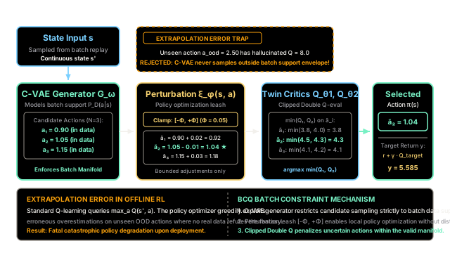
1State s'2   │3   ├─────────────────────────────────────────┐4   ▼                                         ▼5┌─────────────────────────────────┐   ┌─────────────────────────────────┐6│ Conditional VAE Generator G_ω   │   │ Perturbation Network ξ_φ        │7│ Samples N in-distribution {a_i} │   │ Clamped leash: [-Φ, +Φ]         │8└─────────────────────────────────┘   └─────────────────────────────────┘9   │                                         │10   └────────────────────┬────────────────────┘11                        ▼12           Perturbed Actions ã_i = a_i + ξ_φ(s', a_i)13                        │14                        ▼15       ┌─────────────────────────────────┐16       │ Twin Target Critics Q'_1, Q'_2  │17       │ Evaluates: min(Q'_1, Q'_2)      │18       └─────────────────────────────────┘19                        │20                        ▼21      Optimal In-Distribution Action π(s')

1. Generative Model of the Behavior Policy ($G_\omega$)

BCQ fits a Conditional Variational Autoencoder (C-VAE) $G_\omega = (E_{\omega_1}, D_{\omega_2})$ to model the conditional distribution of actions observed in the dataset, $P_\mathcal{D}(a \mid s)$.

• The Encoder $q_{\omega_1}(z \mid s, a)$ maps a state-action pair to a latent Gaussian distribution $\mathcal{N}(\mu(s, a), \sigma^2(s, a))$.
• The Decoder $D_{\omega_2}(s, z)$ reconstructs the action from state $s$ and latent code $z \sim \mathcal{N}(0, I)$.

The C-VAE is trained by maximizing the Evidence Lower Bound (ELBO) on transitions $(s, a) \sim \mathcal{D}$:

$\mathcal{L}_{\text{VAE}}(\omega) = \mathbb{E}_{(s, a) \sim \mathcal{D},\, z \sim q_{\omega_1}} \left[ \|a - D_{\omega_2}(s, z)\|^2 + D_{\text{KL}}\left( q_{\omega_1}(z \mid s, a) \,\parallel\, \mathcal{N}(0, I) \right) \right]$

During policy evaluation, the agent samples $N$ latent vectors $z_i \sim \mathcal{N}(0, I)$ and decodes candidate actions:

$a_i = D_{\omega_2}(s, z_i), \quad i \in \{1, \dots, N\}$

Because the C-VAE was trained solely on dataset $\mathcal{D}$, these $N$ actions are guaranteed to lie within the support of the behavior policy.

2. Perturbation Model ($\xi_\phi$)

Relying purely on the C-VAE would reduce the algorithm to behavioral cloning, preventing the agent from outperforming suboptimal demonstration data. To enable policy optimization while preserving safety, BCQ adds a perturbation network $\xi_\phi(s, a)$:

$\tilde{a} = a + \xi_\phi(s, a), \quad \text{where } \xi_\phi(s, a) = \Phi \tanh\left(\text{MLP}_\phi(s, a)\right)$

The parameter $\Phi$ acts as a strict mathematical "leash" (typically $\Phi = 0.05 \cdot a_{\max}$). The perturbation network can adjust the candidate action by at most $\pm \Phi$, enabling local gradient ascent toward higher returns without drifting into out-of-distribution regions.

The perturbation network is trained to maximize expected $Q$-value:

$\phi \leftarrow \arg\max_\phi \mathbb{E}_{(s, a) \sim \mathcal{D}} \left[ Q_{\theta_1}\left(s, a + \xi_\phi(s, a)\right) \right]$

3. Clipped Double Q-Learning Target

To penalize residual uncertainty within the candidate pool, BCQ evaluates candidate actions using twin target critics $(Q'_{\theta_1}, Q'_{\theta_2})$.

At acting time, the policy chooses the candidate that maximizes the minimum predicted value:

$\pi(s) = \arg\max_{a_i + \xi_\phi(s, a_i)} \min_{j=1,2} Q_{\theta_j}\left(s,\, a_i + \xi_\phi(s, a_i)\right), \quad \text{for } \{a_i\}_{i=1}^N \sim G_\omega(s)$

For the Bellman target update, BCQ computes a convex combination of the minimum and maximum critic predictions:

$y = r + \gamma \max_{a'_i} \left[ \lambda \min_{j=1,2} Q'_{\theta_j}(s', \tilde{a}'_i) + (1 - \lambda) \max_{j=1,2} Q'_{\theta_j}(s', \tilde{a}'_i) \right]$

where $\tilde{a}'_i = a'_i + \xi_\phi(s', a'_i)$ and $\lambda \in [0.75, 1.0]$. Setting $\lambda = 1.0$ yields standard conservative lower-bound estimation.

Worked numerical example

Let us trace a concrete Bellman target evaluation at state $s'$, where the true demonstrated action support lies in the interval $[0.8, 1.2]$, with reward $r = 1.5$, discount factor $\gamma = 0.95$, and conservatism parameter $\lambda = 1.0$.

Step 1: Sample $N=3$ Candidate Actions from C-VAE

The Conditional VAE $G_\omega(s')$ generates $N=3$ samples from the data manifold:

• $a_1 = 0.90$
• $a_2 = 1.05$
• $a_3 = 1.15$

All three candidates reside safely within the demonstrated band $[0.8, 1.2]$.

Step 2: Apply Bounded Perturbation ($\Phi = 0.05$)

The perturbation network $\xi_\phi(s', a)$ evaluates each candidate and outputs local adjustments clamped within $[-0.05, 0.05]$:

• For $a_1 = 0.90$: $\Delta a_1 = +0.02 \implies \tilde{a}_1 = 0.90 + 0.02 = 0.9200$
• For $a_2 = 1.05$: $\Delta a_2 = -0.01 \implies \tilde{a}_2 = 1.05 - 0.01 = 1.0400$
• For $a_3 = 1.15$: $\Delta a_3 = +0.03 \implies \tilde{a}_3 = 1.15 + 0.03 = 1.1800$

Step 3: Evaluate Twin Target Critics

The twin critics $(Q'_{\theta_1}, Q'_{\theta_2})$ evaluate the three perturbed candidates:

• Candidate $\tilde{a}_1 = 0.92$: $Q'_1 = 3.80$, $Q'_2 = 4.00 \implies \min(Q'_1, Q'_2) = 3.8000$
• Candidate $\tilde{a}_2 = 1.04$: $Q'_1 = 4.50$, $Q'_2 = 4.30 \implies \min(Q'_1, Q'_2) = 4.3000$
• Candidate $\tilde{a}_3 = 1.18$: $Q'_1 = 4.10$, $Q'_2 = 4.20 \implies \min(Q'_1, Q'_2) = 4.1000$

Step 4: Batch Constrained Action Selection

The policy selects the candidate that maximizes the conservative minimum:

$\max\{3.8000,\, 4.3000,\, 4.1000\} = 4.3000 \implies \text{Select } \tilde{a}_2 = 1.0400$

Step 5: Compute Bellman Target

Using $\lambda = 1.0$:

$y = r + \gamma \cdot \min_{j=1,2} Q'_j(s', \tilde{a}_2) = 1.5 + 0.95 \times 4.3000 = 1.5 + 4.0850 = 5.5850$

Why This Beats Standard Off-Policy RL

Suppose an unconstrained actor (like DDPG) queried the critic at an out-of-distribution action $a_{\text{ood}} = 2.50$. Due to function approximation error, critic 1 predicts a hallucinated value $Q'_1(s', 2.50) = 8.00$.

An unconstrained algorithm would greedily select $a_{\text{ood}}$ and compute an inflated target of $1.5 + 0.95 \times 8.0 = 9.10$. BCQ completely circumvents this failure mode because $a_{\text{ood}} = 2.50$ is never sampled by the C-VAE, rendering the hallucination harmless.

Code

Below is a self-contained, type-hinted Python implementation of BCQ's candidate generation, perturbation bounding, twin-critic evaluation, and Bellman target calculation:

1from dataclasses import dataclass2import math3from typing import List, Tuple4
5
6@dataclass7class ActionCandidate:8    """Stores candidate action evaluations and conservative value metrics."""9
10    raw_action: float11    perturbation: float12    perturbed_action: float13    q1: float14    q2: float15    conservative_q: float16
17
18class ConditionalVAEGenerator:19    """Simulates a Conditional VAE modeling the batch dataset support P_D(a|s)."""20
21    def sample_candidates(self, state: float, num_samples: int) -> List[float]:22        """Samples candidate actions guaranteed to lie on the demonstrated data manifold."""23        # For state s' = 1.0, generates N=3 samples strictly on the dataset support24        candidate_pool = [0.90, 1.05, 1.15]25        return candidate_pool[:num_samples]26
27
28class PerturbationNetwork:29    """Perturbation model xi_phi(s, a) outputting adjustments bounded by [-Phi, Phi]."""30
31    def __init__(self, phi_limit: float = 0.05) -> None:32        self.phi_limit = phi_limit33
34    def perturb(self, state: float, action: float) -> Tuple[float, float]:35        """Applies clamped perturbation delta bounded strictly by [-phi_limit, phi_limit]."""36        if math.isclose(action, 0.90):37            raw_delta = 0.0238        elif math.isclose(action, 1.05):39            raw_delta = -0.0140        elif math.isclose(action, 1.15):41            raw_delta = 0.0342        else:43            raw_delta = 0.044
45        # Enforce mathematical leash [-Phi, Phi]46        clipped_delta = max(-self.phi_limit, min(self.phi_limit, raw_delta))47        perturbed_action = action + clipped_delta48        return clipped_delta, perturbed_action49
50
51class TwinTargetCritic:52    """Twin Q-networks (Q1', Q2') evaluating state-action pairs."""53
54    def evaluate(self, state: float, action: float) -> Tuple[float, float]:55        """Returns (Q1', Q2') estimates."""56        if math.isclose(action, 0.92):57            return 3.8, 4.058        elif math.isclose(action, 1.04):59            return 4.5, 4.360        elif math.isclose(action, 1.18):61            return 4.1, 4.262        elif math.isclose(action, 2.50):63            # Unconstrained OOD action with hallucinated Q164            return 8.0, 1.565        else:66            return 0.0, 0.067
68
69class BatchConstrainedQLearning:70    """Core decision engine of Batch Constrained Q-Learning (BCQ)."""71
72    def __init__(73        self,74        cvae: ConditionalVAEGenerator,75        perturbation_net: PerturbationNetwork,76        twin_critics: TwinTargetCritic,77        gamma: float = 0.95,78        lam: float = 1.0,79    ) -> None:80        self.cvae = cvae81        self.perturbation_net = perturbation_net82        self.critics = twin_critics83        self.gamma = gamma84        self.lam = lam85
86    def select_action_and_target(87        self, next_state: float, reward: float, num_samples: int = 388    ) -> Tuple[ActionCandidate, float]:89        """Generates candidates from C-VAE, perturbs them within leash,90
91        evaluates twin critics, and computes conservative Bellman target.92        """93        # 1. Sample N candidate actions from C-VAE (confined to batch manifold)94        raw_actions = self.cvae.sample_candidates(next_state, num_samples)95
96        candidates: List[ActionCandidate] = []97        for a in raw_actions:98            delta, a_tilde = self.perturbation_net.perturb(next_state, a)99            q1, q2 = self.critics.evaluate(next_state, a_tilde)100
101            # BCQ evaluation: lambda * min(Q1, Q2) + (1 - lambda) * max(Q1, Q2)102            conservative_q = self.lam * min(q1, q2) + (1.0 - self.lam) * max(103                q1, q2104            )105
106            candidates.append(107                ActionCandidate(108                    raw_action=a,109                    perturbation=delta,110                    perturbed_action=round(a_tilde, 4),111                    q1=q1,112                    q2=q2,113                    conservative_q=conservative_q,114                )115            )116
117        # 2. Select candidate maximizing conservative Q-value118        best_candidate = max(candidates, key=lambda c: c.conservative_q)119
120        # 3. Compute Bellman Target: y = r + gamma * max conservative Q121        target_y = reward + self.gamma * best_candidate.conservative_q122
123        return best_candidate, target_y124
125
126if __name__ == "__main__":127    cvae = ConditionalVAEGenerator()128    perturbation = PerturbationNetwork(phi_limit=0.05)129    critics = TwinTargetCritic()130    bcq = BatchConstrainedQLearning(131        cvae, perturbation, critics, gamma=0.95, lam=1.0132    )133
134    # Execute BCQ selection and Bellman target calculation135    best_action, bellman_y = bcq.select_action_and_target(136        next_state=1.0, reward=1.5, num_samples=3137    )138
139    print("=== BCQ Candidate Action Selection ===")140    print(f"Selected Perturbed Action: {best_action.perturbed_action}")141    print(f"Raw Base Action:          {best_action.raw_action}")142    print(f"Applied Perturbation:     {best_action.perturbation:+.4f}")143    print(f"Critic Q1:                {best_action.q1:.2f}")144    print(f"Critic Q2:                {best_action.q2:.2f}")145    print(f"Conservative min(Q1, Q2): {best_action.conservative_q:.2f}")146
147    print("\n=== Bellman Target Calculation ===")148    print(149        f"Target y = r + gamma * Q_target: 1.5 + 0.95 * {best_action.conservative_q} = {bellman_y:.4f}"150    )151
152    # Exact assertions matching worked numerical example153    assert math.isclose(best_action.perturbed_action, 1.04)154    assert math.isclose(best_action.conservative_q, 4.3)155    assert math.isclose(bellman_y, 5.585)

Expected output:

1=== BCQ Candidate Action Selection ===2Selected Perturbed Action: 1.043Raw Base Action:          1.054Applied Perturbation:     -0.01005Critic Q1:                4.506Critic Q2:                4.307Conservative min(Q1, Q2): 4.308
9=== Bellman Target Calculation ===10Target y = r + gamma * Q_target: 1.5 + 0.95 * 4.3 = 5.5850

Watch Out For

The Quick Version

• Extrapolation Error Prevention: Standard off-policy algorithms fail offline because policy optimization exploits out-of-distribution critic overestimations; BCQ eliminates this by restricting actions to the batch data support.
• Generative Manifold Modeling: A Conditional VAE (C-VAE) learns the behavior policy distribution $P_\mathcal{D}(a \mid s)$, sampling candidate actions guaranteed to reside within the demonstrated dataset.
• Bounded Perturbation Leash: A separate perturbation network $\xi_\phi(s, a)$ adds minor adjustments clamped within $[-\Phi, \Phi]$, allowing the policy to outperform demonstrated behaviors without venturing out-of-distribution.
• Conservative Double Q-Target: BCQ evaluates candidate actions through twin target critics, selecting the candidate that maximizes $\min(Q_1, Q_2)$ to guard against function approximation noise.

What to Read Next

• Offline / Batch Reinforcement Learning
• Conservative Q-Learning (CQL)
• Distributional Shift in Offline RL