Offline / Batch Reinforcement Learning

Why Does This Exist?

In classic online reinforcement learning, an agent learns through active trial and error: it executes actions in the environment, observes the consequences, and collects new experiences to correct its mistakes.

However, in many real-world domains, active online exploration is dangerous, unethical, or economically impossible:

• Healthcare: A clinical policy cannot experiment with random medication dosages on critically ill patients just to see what happens.
• Autonomous Driving: A vehicle control algorithm cannot test what happens when driving into a highway divider.
• Industrial Process Control & Nuclear Power: Operating a chemical refinery or nuclear reactor outside calibrated safety margins causes catastrophic physical destruction.
• High-Frequency Trading: A flawed exploratory trading strategy can wipe out millions of dollars within milliseconds.

In each of these industries, organizations possess massive archives of historical operational data collected by past human operators, legacy rule-based controllers, or sub-optimal policies:

Offline reinforcement learning (also called Batch RL; Lange et al., 2012; Levine et al., 2020) solves this challenge by training policies strictly from static datasets $\mathcal{D}$ with zero environment interaction during training.

Why Standard Off-Policy RL Fails Offline

Standard deep Q-learning methods (DQN, DDPG, SAC) are theoretically "off-policy"—their Bellman error equations do not mandate that data come from the current policy. Yet when practitioners execute standard SAC or DQN directly on an offline dataset, the algorithms collapse completely.

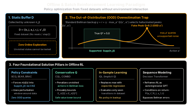
Without online interaction to verify actions, standard temporal difference updates query unobserved, out-of-distribution (OOD) actions. The maximization operator ($\max_{a'} Q(s', a')$) latches onto positive neural network generalization errors, creating an escalating spiral of delusion that destroys policy performance.

Think of It Like This

How It Actually Works

The OOD Action Maximization Trap and Solution Taxonomy

In standard temporal difference learning, the target value for updating the action-value function $Q_\theta(s, a)$ is given by the Bellman optimality operator:

When training online, if the function approximator assigns an erroneously high $Q$-value to an action $a'$, the agent will subsequently execute $a'$ in the environment. The real environment returns a low reward, and the network immediately corrects the error.

In the offline setting, the agent cannot collect new data to refute false beliefs. The failure unfolds in three cascading steps:

11. Out-of-Distribution Query:2   Target state s' has actions a' NOT supported by behavior policy π_β (density π_β(a' | s') ≈ 0).3
42. Maximization Bias Over Extrapolation Errors:5   Q_θ(s', a') has high epistemic variance in OOD regions.6   The max operator naturally selects max_a' Q_θ(s', a'), picking the highest positive noise spike!7
83. Compounding Delusion:9   Target y = r + γ · max Q(s', a') becomes massively inflated.10   Subsequent Bellman backups propagate this hallucinated value to preceding states, collapsing the policy.

The Four Algorithmic Solution Pillars

Modern offline reinforcement learning resolves the OOD overestimation trap through four primary algorithmic paradigms:

1. Policy Constraint Methods (BCQ, BEAR, BRAC)

These methods constrain the learned policy $\pi_\theta(a \mid s)$ to only select actions within the support of the behavior policy $\pi_\beta(a \mid s)$:

Batch-Constrained Q-learning (BCQ) trains a conditional Variational Autoencoder (VAE) to model $p(a \mid s)$ under $\pi_\beta$, then samples candidate actions strictly from the VAE and applies a small bounded perturbation $\xi_\phi(s, a)$.

2. Conservative Value Penalties (CQL, COMBO)

Rather than constraining the policy, Conservative Q-Learning (CQL) modifies the value function loss to explicitly penalize $Q$-values for out-of-distribution actions while maximizing $Q$-values on dataset actions:

CQL mathematically guarantees that the expected value under the learned policy lower-bounds the true value:

3. In-Sample Learning (IQL)

Implicit Q-Learning (IQL) completely avoids querying counterfactual out-of-distribution actions during Bellman updates. It fits the value function $V_\psi(s)$ using asymmetric expectile regression purely over actions present in the dataset:

Setting $\tau \in [0.7, 0.9]$ computes an upper-expectile that approximates $\max_{a \in \mathcal{D}} Q(s, a)$ strictly inside the data support.

4. Trajectory Sequence Modeling (Decision Transformer)

Reframes offline RL as conditional autoregressive sequence modeling. Using standard GPT architectures, Decision Transformer (DT) models trajectories as sequences of tokens:

At test time, the user conditions the transformer on a desired return-to-go $\hat{R}_1 = \sum_{t=1}^T r_t$, and the model autoregressively generates actions that achieve that return without any temporal difference updates or value functions.

Worked numerical example

Let us trace a single transition update under standard Q-learning versus Conservative Q-learning (CQL) in the presence of out-of-distribution extrapolation errors.

Setup:

• Current state transition: $(s, a, r, s')$ with immediate reward $r = 1.0$ and discount $\gamma = 0.9$.
• Next state $s'$ has 3 discrete candidate actions $\{a_{\text{data}}, a_{\text{ood1}}, a_{\text{ood2}}\}$.
• The dataset $\mathcal{D}$ only contains observations for $a_{\text{data}}$.
• True optimal value: $Q^*(s', a_{\text{data}}) = 5.0$.
• Neural network function approximator outputs:
  • Supported action: $Q(s', a_{\text{data}}) = 5.0$ (accurate calibration on data).
  • Out-of-distribution action 1: $Q(s', a_{\text{ood1}}) = 9.2$ (positive extrapolation spike).
  • Out-of-distribution action 2: $Q(s', a_{\text{ood2}}) = 2.1$ (negative extrapolation spike).

Step 1: Standard Q-Learning Bellman Target

Standard Q-learning executes unconstrained maximization across all action heads:

Target calculation:

• Ground-truth target supported by data: $y^* = 1.0 + 0.9(5.0) = 5.50$.
• Target overestimation error: $$\Delta_{\text{target}} = y_{\text{std}} - y^* = 9.28 - 5.50 = +3.78$$
• The network updates $Q(s, a)$ toward $9.28$, hallucinating an inflated return driven purely by ungrounded noise on $a_{\text{ood1}}$.

Step 2: Conservative Q-Learning (CQL) Target

CQL applies an explicit conservatism penalty $\alpha = 5.0$ to actions unsupported by the dataset $\mathcal{D}$:

Evaluating each candidate action:

• $\tilde{Q}(s', a_{\text{data}}) = 5.0$ (supported in $\mathcal{D}$)
• $\tilde{Q}(s', a_{\text{ood1}}) = 9.2 - 5.0 = 4.2$ (penalized OOD spike)
• $\tilde{Q}(s', a_{\text{ood2}}) = 2.1 - 5.0 = -2.9$ (penalized OOD)

Conservative action selection:

Target calculation:

• CQL successfully suppresses the hallucinated peak on $a_{\text{ood1}}$ ($4.2 < 5.0$).
• Target error: $y_{\text{CQL}} - y^* = 5.50 - 5.50 = 0.00$. The Bellman target remains grounded in verified transition data.

Code

1from dataclasses import dataclass2from typing import List, Tuple3
4
5@dataclass6class ActionEvaluation:7    """Represents a candidate action evaluation under an offline Q-function."""8
9    name: str10    is_in_dataset: bool11    predicted_q: float12
13
14class OfflineBellmanEvaluator:15    """Demonstrates the vulnerability of standard Q-learning to OOD actions16
17    and how Conservative Q-Learning (CQL) eliminates overestimation bias.18    """19
20    def __init__(self, gamma: float = 0.9, cql_penalty: float = 5.0) -> None:21        self.gamma = gamma22        self.cql_penalty = cql_penalty23
24    def compute_standard_target(25        self,26        reward: float,27        candidates: List[ActionEvaluation],28    ) -> Tuple[float, str, float]:29        """Calculates standard Q-learning target: y = r + gamma * max_a' Q(s', a')."""30        best_candidate = max(candidates, key=lambda c: c.predicted_q)31        target = reward + self.gamma * best_candidate.predicted_q32        return target, best_candidate.name, best_candidate.predicted_q33
34    def compute_conservative_target(35        self,36        reward: float,37        candidates: List[ActionEvaluation],38    ) -> Tuple[float, str, float]:39        """Calculates conservative Q target: penalizes out-of-distribution action peaks."""40        penalized_scores = []41        for c in candidates:42            adjusted_q = (43                c.predicted_q44                if c.is_in_dataset45                else c.predicted_q - self.cql_penalty46            )47            penalized_scores.append((c.name, adjusted_q))48
49        best_name, best_q = max(penalized_scores, key=lambda item: item[1])50        target = reward + self.gamma * best_q51        return target, best_name, best_q52
53
54# Test scenario matching the worked numerical example55evaluator = OfflineBellmanEvaluator(gamma=0.9, cql_penalty=5.0)56reward = 1.057
58# Q-values predicted by a neural network with unconstrained OOD extrapolation59actions = [60    ActionEvaluation(61        name="a_data", is_in_dataset=True, predicted_q=5.062    ),  # True support63    ActionEvaluation(64        name="a_ood1", is_in_dataset=False, predicted_q=9.265    ),  # Hallucinated spike66    ActionEvaluation(67        name="a_ood2", is_in_dataset=False, predicted_q=2.168    ),  # Negative spike69]70
71# 1. Standard Q-learning calculation72y_std, best_std_name, q_std = evaluator.compute_standard_target(reward, actions)73print(74    f"Standard Target: {y_std:.2f} (selected {best_std_name} with Q={q_std:.1f})"75)76# -> Standard Target: 9.28 (selected a_ood1 with Q=9.2)77
78# 2. Conservative Q-learning calculation79y_cql, best_cql_name, q_cql = evaluator.compute_conservative_target(80    reward, actions81)82print(83    f"Conservative Target: {y_cql:.2f} (selected {best_cql_name} with Q={q_cql:.1f})"84)85# -> Conservative Target: 5.50 (selected a_data with Q=5.0)86
87# 3. Ground truth evaluation88true_grounded_target = reward + 0.9 * 5.089overestimation_error = y_std - true_grounded_target90cql_error = y_cql - true_grounded_target91
92print(f"Standard Overestimation Error: +{overestimation_error:.2f}")93# -> Standard Overestimation Error: +3.7894
95print(f"Conservative Target Error: {cql_error:.2f}")96# -> Conservative Target Error: 0.0097
98# Verification assertions99assert round(y_std, 2) == 9.28100assert best_std_name == "a_ood1"101assert round(y_cql, 2) == 5.50102assert best_cql_name == "a_data"103assert round(overestimation_error, 2) == 3.78104assert round(cql_error, 2) == 0.00

Watch Out For

The Quick Version

• Offline / Batch RL trains optimal decision policies strictly from fixed, pre-collected datasets $\mathcal{D} \sim \pi_\beta$ with zero online simulator or environment interaction.
• Standard off-policy methods collapse offline because the Bellman $\max_{a'}$ operator queries out-of-distribution (OOD) actions, compounding positive neural network extrapolation errors.
• The four foundational offline RL pillars are Policy Constraints (BCQ, BEAR), Conservative Value Penalties (CQL), In-Sample Learning (IQL), and Sequence Modeling (Decision Transformer).
• Unlike Behavioral Cloning, offline RL performs trajectory stitching, discovering optimal policies by recombining the best sub-sequences across heterogeneous sub-optimal demonstrations.

What to Read Next

• Distributional Shift in Offline RL
• Batch Constrained Q-Learning (BCQ)
• Offline Reinforcement Learning
• Decision Transformers and Trajectory Transformer