Distributional Shift in Offline RL
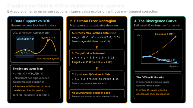
Offline RL trains on static datasets without live exploration, causing Bellman maximization to latch onto uncorrected out-of-distribution overestimations that ruin policy performance.
Why Does This Exist?
The core promise of Offline RL (also known as batch RL) is transformative: train high-performing decision-making agents entirely from pre-collected, static datasets without requiring active trial-and-error exploration. This paradigm is critical for domains where exploration is prohibitively dangerous or expensive, such as autonomous driving, clinical healthcare, financial trading, and heavy industrial automation.
However, applying standard off-policy algorithms like Deep Q-Networks (DQN) or Soft Actor-Critic (SAC) directly to static datasets leads to catastrophic failure. When evaluated in the real environment, policies trained naively offline frequently achieve returns far worse than the average data-collection policy—often collapsing completely to zero.
The fundamental culprit is distributional shift. In supervised learning, testing a neural network on out-of-distribution (OOD) inputs leads to poor predictions, but those errors remain localized and benign. In reinforcement learning, however, value iteration is dynamic and auto-regressive:
- The policy attempts to improve beyond the data-collection behavior policy , searching for actions with higher predicted returns.
- When querying the Q-function on unseen action candidates , deep neural networks exhibit unpredictable, high-variance extrapolation behavior.
- The Bellman target operator queries a greedy maximization: . If the network happens to overestimate the value of even a single unseen action, the operator immediately latches onto that hallucinated peak.
- Because the agent cannot interact with the physical environment to collect real feedback and correct its mistake, this erroneous target trains predecessor states, cascading backwards through the state graph like an unchecked contagion.
Without explicit algorithmic mechanisms to constrain policy choices or penalize out-of-distribution values, offline Q-learning inevitably succumbs to The Deadly Triad: function approximation, bootstrapping, and off-policy training without corrective feedback.
Think of It Like This
A Flight Control AI Trained Only in Calm Skies
Picture a deep neural network trained to pilot commercial aircraft, trained entirely on a static flight recorder dataset recorded by seasoned pilots flying through calm, sunny weather.
During offline training, the algorithm tries to learn an optimal autopilot policy. The neural network encounters a simulated turbulence scenario. Because the dataset contains zero examples of high-altitude wing stalls, the neural network's unconstrained function approximator happens to assign an astronomical value () to pitching the aircraft's nose upward at 75 degrees into a full aerodynamic stall. In the mathematical imagination of the network, this radical pitch maneuver is predicted to produce a silky-smooth glide.
In an online simulator, the autopilot would attempt this pitch, stall the wings, crash, receive a reward, and immediately learn to never pitch up. The error would be snuffed out in a single step.
In offline RL, there is no physical flight test. The Bellman update takes this hallucinated value as absolute truth. It concludes that pitching up into a stall is the ultimate life-saving procedure and reinforces every upstream decision leading into it. When deployed on a physical plane in real turbulence, the autopilot executes the stall at the first wind gust, destroying the aircraft.
Where the analogy stops: A human pilot has aerodynamic domain knowledge and physical common sense. A deep neural network has no innate physical understanding; it is simply a high-dimensional function approximator whose outputs outside the training manifold are arbitrary mathematical artifacts.
How It Actually Works
Covariate Shift vs. Value Extrapolation Error
Distributional shift in offline reinforcement learning consists of two interconnected mechanisms formalized by Levine et al. (2020), Fujimoto et al. (2019), and Kumar et al. (2020):
+-----------------------------------------------------------------------+| 1. State-Action Covariate Shift || Behavior Policy pi_beta !===> Learned Target Policy pi || Data Support: d^{pi_beta}(s, a) =/= State Visitation: d^pi(s, a) |+-----------------------------------------------------------------------+ | v+-----------------------------------------------------------------------+| 2. Extrapolation Error (OOD Value Delusion) || Target: y = r + gamma * max_{a'} Q_theta(s', a') || Unseen action a_ood yields random positive error: Q_theta >> Q* |+-----------------------------------------------------------------------+ | v+-----------------------------------------------------------------------+| 3. Unchecked Bellman Error Contagion || Max latches onto a_ood ---> Predecessor target y explodes || No environment feedback ---> Q-values -> 10^6, Real Return -> 0 |+-----------------------------------------------------------------------+1. State-Action Covariate Shift
The static dataset was collected by one or more behavior policies , inducing a state-action marginal distribution . The goal of offline RL is to find a superior policy . Consequently, the state-action visitation distribution of the target policy drifts away from the dataset support:
As the policy deviates, it queries the action-value function on state-action pairs where the empirical data density .
2. Extrapolation Error (OOD Value Delusion)
In standard Q-learning, the Bellman optimality target is:
In continuous actor-critic methods, the target takes the expectation under the actor :
Because deep neural networks do not generalize uniformly to unvisited domains, evaluating on an unseen action produces arbitrary values. The actor's objective is explicitly designed to maximize the Q-function:
The optimizer acts as an adversarial search engine: out of the entire continuous action space, it actively hunts for whatever out-of-distribution action produces the highest positive estimation error.
The Bellman Contagion and Divergence Bounds
In standard online RL, positive extrapolation error is self-correcting. If the agent overestimates , it takes action , observes the real transition , and computes a large negative temporal difference error:
This negative error instantly depresses the overestimated Q-value.
In offline RL, the agent never executes in the environment. The poisoned target is used to update the predecessor state . Because the dataset is repeatedly traversed over thousands of gradient steps, the error circulates through the Bellman equations indefinitely.
The theoretical upper bound on compounding error across iterations of offline fitted Q-iteration satisfies:
where represents the extrapolation gap.
Notice that the extrapolation error compounds across the effective horizon . In empirical benchmarks, this causes the deadly divergence curve: the neural network's estimated Q-values explode to or ("delusional optimism"), while the real-world return of the policy plunges to zero upon physical deployment.
Worked numerical example
Let us trace a concrete 2-step chain MDP to demonstrate how a single out-of-distribution action poisons the entire value landscape:
- MDP Topology:
- Predecessor state : Taking action yields reward and transitions deterministically to next state .
- Next state : Has two available actions:
- (observed in data): True environmental value .
- (unseen in data, catastrophic): True environmental value .
- Discount factor: .
- Static Dataset :
- Contains transitions: and .
- Contains zero examples of .
- Neural Network Initial Estimates:
- For dataset action: (accurately fitted from data).
- For unseen action: Due to random weight initialization and function approximation noise, .
Step 1: Compute the Bellman Target for Predecessor Under standard unconstrained Q-learning, the Bellman backup evaluates the greedy maximum over all actions at next state :
The target value for predecessor state becomes:
Step 2: Quantify the Target Overestimation Error The true return under the optimal feasible policy should be:
The overestimation injected into state is:
Step 3: Policy Optimization Delusion When the policy at state is updated to maximize predicted Q-values:
The policy firmly commits to the out-of-distribution action because the network falsely promises a return of .
Step 4: Physical Deployment Collapse When deployed in the real environment, the agent reaches and executes . The actual physical return achieved from is:
Comparing the perceived versus physical outcome:
- Perceived (Estimated) Value:
- Actual Realized Return:
- Performance Collapse: A drop in performance caused by a single unvisited action. Over multiple training iterations, this error cascades backward to earlier states, inflating values while real performance plummets.
Code
import numpy as np
class OfflineDistributionalShiftSimulator: """Simulates the mechanism of extrapolation error and value divergence
in offline Q-learning contrasted with data-support constrained updates. """
def __init__(self, gamma: float = 0.9) -> None: self.gamma = gamma # Ground-truth environment returns self.true_q = {"a_dataset": 2.0, "a_ood": 0.5} self.r_predecessor = 1.0
def run_unconstrained_bellman_step( self, q_estimates: dict[str, float] ) -> tuple[float, float, str, float]: """Simulates standard unconstrained Q-learning Bellman backup from predecessor state s_0.""" # Policy chooses greedy action at next state s_1 chosen_action = max(q_estimates, key=q_estimates.get) max_q_next = q_estimates[chosen_action]
# Target for predecessor state s_0 target_s0 = self.r_predecessor + self.gamma * max_q_next
# True return if executing chosen action in physical environment true_return_s0 = ( self.r_predecessor + self.gamma * self.true_q[chosen_action] ) overestimation = target_s0 - ( self.r_predecessor + self.gamma * self.true_q["a_dataset"] )
return target_s0, true_return_s0, chosen_action, overestimation
def simulate_compounding_divergence( self, num_iterations: int = 10, noise_factor: float = 0.5 ) -> list[tuple[int, float, float]]: """Simulates compounding Q-value explosion across offline backup iterations.""" # Initial estimate at s_1: OOD action has initial positive error q_ood = 3.5 history: list[tuple[int, float, float]] = []
curr_q = q_ood for i in range(1, num_iterations + 1): # In offline training without correction, max operator latches onto OOD error target = self.r_predecessor + self.gamma * curr_q history.append((i, curr_q, target)) # OOD noise continues to compound as network fits inflated targets curr_q = target + noise_factor
return history
def run_constrained_bellman_step( self, q_estimates: dict[str, float] ) -> tuple[float, float, str, float]: """Simulates constrained offline Q-learning (restricting max to dataset support).""" # Constraint: policy can only select actions with dataset support chosen_action = "a_dataset" constrained_q_next = q_estimates[chosen_action]
target_s0 = self.r_predecessor + self.gamma * constrained_q_next true_return_s0 = ( self.r_predecessor + self.gamma * self.true_q[chosen_action] ) overestimation = target_s0 - true_return_s0
return target_s0, true_return_s0, chosen_action, overestimation
if __name__ == "__main__": np.set_printoptions(precision=4, suppress=True)
sim = OfflineDistributionalShiftSimulator(gamma=0.9)
# Initial estimates matching worked numerical example q_initial = {"a_dataset": 2.0, "a_ood": 3.5}
# Step 1: Unconstrained Bellman backup target_unconstrained, return_unconstrained, action_unconstrained, err = ( sim.run_unconstrained_bellman_step(q_initial) )
# Step 2: Constrained Bellman backup (data-support constraint) ( target_constrained, return_constrained, action_constrained, err_constrained, ) = sim.run_constrained_bellman_step(q_initial)
# Step 3: Compounding divergence over 10 iterations divergence_history = sim.simulate_compounding_divergence( num_iterations=10, noise_factor=0.5 )
print(f"Unconstrained Target y(s_0, a_0): {target_unconstrained:.2f}") # -> Unconstrained Target y(s_0, a_0): 4.15
print(f"Chosen Action at s_1: {action_unconstrained}") # -> Chosen Action at s_1: a_ood
print(f"Target Overestimation Error: +{err:.2f}") # -> Target Overestimation Error: +1.35
print(f"Actual Return upon Deployment: {return_unconstrained:.2f}") # -> Actual Return upon Deployment: 1.45
print(f"Constrained Target y(s_0, a_0): {target_constrained:.2f}") # -> Constrained Target y(s_0, a_0): 2.80
print(f"Constrained Actual Return: {return_constrained:.2f}") # -> Constrained Actual Return: 2.80
print( f"Compounding Divergence at iteration 10: Q = {divergence_history[-1][1]:.2f}" ) # -> Compounding Divergence at iteration 10: Q = 10.54
# Assert correctness assert np.isclose(target_unconstrained, 4.15, atol=1e-2) assert action_unconstrained == "a_ood" assert np.isclose(err, 1.35, atol=1e-2) assert np.isclose(return_unconstrained, 1.45, atol=1e-2) assert np.isclose(target_constrained, 2.80, atol=1e-2) assert np.isclose(return_constrained, 2.80, atol=1e-2) assert divergence_history[-1][1] > 10.0Watch Out For
Assuming More Offline Training Epochs Resolves Extrapolation Error
In supervised learning, training a neural network for more epochs on a fixed dataset decreases training loss and typically refines decision boundaries. Practitioners transitioning to offline reinforcement learning often assume that when policy performance is poor, the network simply needs more gradient steps over the offline dataset.
In offline RL, this assumption is disastrously false. The neural network only receives gradient supervision on in-distribution tuples . Unseen out-of-distribution actions receive zero negative gradient updates. As training epochs increase:
- The network's weights specialize, increasing the Lipschitz roughness of the function approximator.
- Unconstrained ridges and extreme spikes in the OOD action landscape become sharper and taller.
- The Bellman backup recirculates inflated targets more times through the replay buffer, actively accelerating value divergence.
Consequently, training for more epochs without constraints widens the extrapolation gap and degrades real-world performance faster.
The Fix: Never use raw Bellman training loss or TD error to judge convergence in offline RL. Instead:
- Apply Policy Constraints: Constrain the learned policy to stay within the support of the behavior policy (e.g., Batch-Constrained Q-Learning / BCQ or KL-divergence penalties).
- Apply Value Regularization: Use Conservative Q-Learning (CQL) to penalize Q-values on out-of-distribution actions, guaranteeing that remains a conservative lower bound on true returns.
- Use In-Sample Learning: Adopt Implicit Q-Learning (IQL), which avoids querying the Q-network on unseen actions entirely by using expectile regression over dataset transitions.
- Evaluate with Off-Policy Evaluation (OPE): Validate policy quality using Fitted Q Evaluation (FQE) or Doubly Robust estimators rather than trusting raw Q-network predictions.
The Quick Version
- Absence of Corrective Feedback: Unlike online RL where taking a bad action immediately penalizes the agent, offline RL operates on static data with no physical environment to disprove hallucinated returns.
- Maximization Latch: The Bellman operator acts as an adversarial filter, consistently selecting out-of-distribution actions that have accidental positive extrapolation errors.
- Backward Error Propagation: Overestimated target values cascade backward into predecessor states, creating a positive feedback loop that inflates values across the entire state graph.
- The Divergence Paradox: Training longer on a static dataset exacerbates extrapolation error; preventing policy collapse requires explicit data-support constraints (BCQ), conservative value penalties (CQL), or in-sample evaluation (IQL).