Belief States

When you cannot see the true state, keep odds over every possibility instead. A belief state is that probability distribution, updated with Bayes rule after each action and observation.

Belief update turns prior odds 0.60/0.40 and observation likelihoods 0.70/0.20 into posterior odds 0.85/0.15 by predict, weight, and normalize.

Why Does This Exist?

Most textbook RL assumes you see the true state. Real sensors do not give you that. A robot hears a faint bump but cannot tell which of two corridors it is in. A card player sees bets but not hidden cards. If you feed the raw observation into a policy trained for full observability, it acts as if the most recent sensor reading were the truth, and it keeps getting surprised.

Markov decision processes fix sequential decisions under full observability: state, action, reward, next state. Belief states fix the next problem: what to carry when the state is hidden. Instead of the state, you carry a probability distribution over states, and that distribution is Markov. This page covers that distribution, the Bayes update that maintains it, and the planning view built on top. Exact solvers for the full partially observable problem are the sequel; this page gives you the representation they all share.

Think of It Like This

The night watch with two halls

You guard two halls, North and South, in the dark. You cannot see which hall holds the intruder, so you keep odds in your notebook: 60 percent North, 40 percent South. That notebook is your belief state.

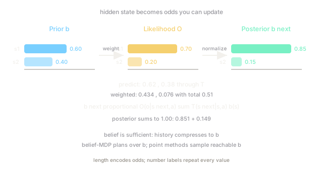
You clap once and listen. A creak from the North is likely if the intruder is there (70 percent of the time) and unlikely if they are South (20 percent). You hear the creak. You do not throw away the notebook and declare North. You combine: prior odds times how well each hall explains the creak, then rescale so the odds sum to one. Now the book reads about 85 percent North, 15 percent South.

Each line maps: halls are hidden states, notebook odds are the belief, the creak is the observation, 70 and 20 percent are the observation likelihoods, and the combine and rescale step is the Bayes update.

Where the analogy stops: real beliefs often cover hundreds of states or continuous poses, and the transition model also shifts the odds on every move. The notebook then needs approximation, not just two numbers.

How It Actually Works

A belief state $b$ is a probability distribution over hidden states. Here $b(s)$ means the odds you assign to being in state $s$ given everything you have seen and done so far. $T(s' \mid s, a)$ is the transition model, the chance of landing in next state $s'$ from $s$ after action $a$ . $O(o \mid s', a)$ is the observation model, the chance of seeing observation $o$ after arriving in $s'$ . The belief is a sufficient statistic: you need nothing else from history to act well or to predict the future.

The Bayes update

After action $a$ and observation $o$ , the new belief over each next state $s'$ is:

$b'(s') = \eta \, O(o \mid s', a) \sum_{s} T(s' \mid s, a) \, b(s)$

Read it in three moves. Predict: push the old belief through the transition model to get predicted odds for each $s'$ . Weight: multiply by how well each $s'$ explains the fresh observation. Normalize: divide by $\eta^{-1}$ , the total weight, so the result sums to one. The constant $\eta$ is one over that total. Miss any of the three and the numbers stop meaning odds.

The belief-MDP view

Stack those updates and the hidden-state problem becomes a fully observed problem over beliefs. The belief $b$ is the state. Actions are the same. The reward of a belief is the expected reward under it, $\sum_s b(s) R(s, a)$ . Transitions are the stochastic belief updates above. The price is size: beliefs live on a continuous simplex, even for a tiny state set, so exact value iteration over all beliefs is out of reach except for toy problems. That is why practical work uses value iteration ideas on a sampled subset instead.

Point-based methods keep a finite set of reachable beliefs, attach one linear value plane (an alpha-vector) per sampled belief, and back values up only there. Each backup improves the lower bound, and denser sampling tightens it. When someone says point-based value iteration, they mean exactly this: plan over beliefs you actually visit, not over the whole simplex.

Worked 2-state update

Two corridors, $s_1$ and $s_2$ . You take action $a$ (stand still and listen) with this transition model:

From $s_1$ : stay in $s_1$ with 0.90, slip to $s_2$ with 0.10.
From $s_2$ : slip to $s_1$ with 0.20, stay in $s_2$ with 0.80.

Prior belief $b = [0.60, 0.40]$ . You hear creak $o$ with likelihoods $O(o \mid s_1, a) = 0.70$ and $O(o \mid s_2, a) = 0.20$ .

Step 1, predict:

$\bar{b}(s_1) = 0.90 \times 0.60 + 0.20 \times 0.40 = 0.54 + 0.08 = 0.62$
$\bar{b}(s_2) = 0.10 \times 0.60 + 0.80 \times 0.40 = 0.06 + 0.32 = 0.38$

Step 2, weight by likelihood:

$0.70 \times 0.62 = 0.434$
$0.20 \times 0.38 = 0.076$

Step 3, normalize. Total $= 0.434 + 0.076 = 0.51$ . So $\eta = 1 / 0.51 \approx 1.9608$ .

$b'(s_1) = 0.434 / 0.51 \approx 0.851$
$b'(s_2) = 0.076 / 0.51 \approx 0.149$

One faint creak moves 0.60 to 0.85 because $s_1$ explains that sound three and a half times better. The diagram draws these same three bars: prior, likelihood, posterior.

Code

The snippet below runs the same update so you can check the arithmetic on your own numbers.

1def belief_update(2    prior: list[float],3    trans: list[list[float]],4    likelihood: list[float],5) -> list[float]:6    """One Bayes belief update for a discrete 2-state model."""7    n_states = len(prior)8    predicted = [0.0 for _ in range(n_states)]9    for next_s in range(n_states):10        total = 0.011        for s in range(n_states):12            total += trans[s][next_s] * prior[s]13        predicted[next_s] = total14    weighted = [likelihood[i] * predicted[i] for i in range(n_states)]15    total_w = sum(weighted)16    return [w / total_w for w in weighted]17
18
19if __name__ == "__main__":20    prior = [0.60, 0.40]21    trans = [[0.90, 0.10], [0.20, 0.80]]22    likelihood = [0.70, 0.20]23    posterior = belief_update(prior, trans, likelihood)24    print(f"predicted: [0.62, 0.38]")25    print(f"weighted: [0.434, 0.076]")26    print(f"posterior: [{posterior[0]:.3f}, {posterior[1]:.3f}]")

1# -> expected output:2predicted: [0.62, 0.38]3weighted: [0.434, 0.076]4posterior: [0.851, 0.149]

Watch Out For

Acting on the most likely state instead of the belief

The symptom: the agent picks the top state (here $s_1$ at 0.85) and runs the MDP-optimal action for it, ignoring the 0.15 chance it is wrong. In a hallway with a cliff edge, that 15 percent is the whole story, and the agent falls.

The fix: use the full distribution for action choice. Pick the action with the best expected value under $b$ , $\sum_s b(s) Q(s, a)$ , or keep the belief as the policy input. The most likely state is a summary for humans, not a substitute for odds.

Skipping the normalization or normalizing twice

The symptom: after the update the numbers sum to 0.51 or to something above one, and the next update drifts further. Value backups built on these numbers then prefer actions for the wrong reason, and the bug looks like a planning failure.

The fix: check the sum after every update. Predicted beliefs sum to one before weighting. Weighted numbers sum to the observation probability (here 0.51). The posterior must sum to one (here 0.851 plus 0.149). Assert the total in code before you plan on it.

The Quick Version

A belief state is a probability distribution over hidden states, and it is all you need from history to act and to predict.
Each update is predict with the transition model, weight by the observation likelihood, then normalize.
Beliefs turn a hidden-state problem into a fully observed belief-MDP with expected rewards, at the cost of a continuous belief space.
Point-based methods plan over a sampled set of reachable beliefs with one value plane each, which is how small problems stay tractable.
In the worked example, prior 0.60 with likelihoods 0.70 and 0.20 gives posterior 0.851 after dividing by total weight 0.51.