Coarse Coding in RL
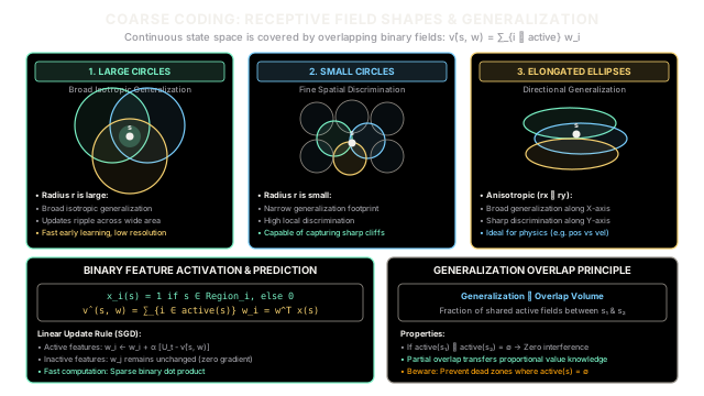
Coarse coding represents continuous state spaces using overlapping binary receptive fields, mapping any state to the set of regions containing it. The geometric shape, size, and orientation of these receptive fields directly sculpt how value knowledge generalizes across the state space.
Why Does This Exist?
In reinforcement learning with continuous state spaces, linear function approximation is widely favored for its theoretical stability, rapid computation, and absence of local optima. However, a linear model can only represent complex, non-linear value surfaces if the feature vector captures non-linear properties of the underlying state space.
If an agent simply passes raw state coordinates (such as ), the linear model can only represent a flat, tilted plane. It cannot represent peaks, valleys, boundaries, or sharp cliffs. Conversely, if the state space is discretized into rigid, non-overlapping grid cells (a tabular histogram), the agent loses all ability to generalize between adjacent cells.
Coarse coding solves this feature engineering challenge by covering the continuous state space with an ensemble of overlapping geometric regions, known as receptive fields.
Each receptive field corresponds to a single binary feature in the representation:
Because the regions overlap, any continuous state activates a whole subset of receptive fields. Updating the weight of an active feature following a transition at state transfers value to every other state that shares that receptive field. Crucially, coarse coding reveals a foundational machine learning insight: the geometric shape, size, and orientation of the receptive fields directly determine how value knowledge generalizes across the state space.
Think of It Like This
Cellular Tower Coverage Zones
Imagine tracking the geographic location of a smartphone across a city:
- The Tabular Approach (GPS Coordinate Memorization): You record the exact latitude and longitude down to six decimal places (e.g.,
(37.774929, -122.419416)). If the phone takes a single step forward, the coordinate changes, and a tabular system treats it as an entirely unknown location with zero signal history. - The Coarse Coding Approach (Overlapping Cellular Towers): The city is covered by overlapping broadcast circles emitted by cellular towers. At any given physical street corner, your phone's receiver detects signals from a specific combination of towers—for example, Tower 3 (Downtown North), Tower 7 (Financial District), and Tower 12 (Bridge Span).
- Your Location Code: Your position is encoded as a binary bitmask indicating active towers:
- Generalization: If lightning strikes and impairs Tower 7, the parameter weights associated with Tower 7 are updated. Anyone standing nearby who also connects to Tower 7 immediately inherits that updated estimate—even if they are standing blocks away on an unvisited side street. The degree of shared signal between two citizens is strictly proportional to how many cell tower circles they share.
Where the analogy breaks down: Cellular radio power falls off smoothly as a continuous inverse-square function of distance. Classic coarse coding uses hard binary cutoff boundaries ()—either you are inside the receptive field or outside it. (Smoothing these boundaries yields Radial Basis Functions). Furthermore, cell towers exist in physical 2D or 3D space, whereas coarse coding can be constructed over arbitrary multi-dimensional physical state spaces (e.g., position, velocity, angle, and angular velocity).
How It Actually Works
Binary Receptive Fields and Generalization Geometry
Coarse coding transforms a continuous state vector into a high-dimensional, sparse binary feature vector .
1. Mathematical Formulation
Let denote a collection of receptive fields defined over the continuous state space . The -th feature is defined as:
The approximate value function is the inner product of the weight vector and feature vector :
where is the set of indices of all receptive fields containing state . The value of state is simply the sum of weights of all receptive fields covering that state.
2. The Linear Semi-Gradient Update
When an agent observes an experience target (such as a Monte Carlo return or a one-step TD target ), the semi-gradient stochastic gradient descent update is:
Because is linear, the gradient with respect to is simply the binary feature vector itself: .
Denoting the TD error as :
- For inactive features (, where ): (no update).
- For active features (, where ):
(Optionally, the step size can be normalized by the number of active features: , ensuring that total value adjustments remain invariant to feature count).
3. How Receptive Field Geometry Dictates Generalization
The geometric characteristics of the receptive fields determine how the learning update at spreads to other states :
LARGE CIRCLES SMALL CIRCLES ELONGATED ELLIPSES ╭─────╮ ╭─╮ ╭─╮ ╭───────────╮ ╭─┤ ├─╮ ╭┤ ├─╮╭┤ ├─╮ ╭┤ ├─╮ │ │ s │ │ │╰─╯ ││╰─╯ │ ││ s ││ ╰─┤ ├─╯ ╰─┬──╯╰──┬─╯ ╰┤ ├─╯ ╰─────╯ ╰─╮ ╭─╯ ╰───────────╯Broad Isotropic Sharp Spatial Directional BiasGeneralization Discrimination (e.g., Position vs Velocity)- Large Receptive Fields (Broad Generalization): When fields have a large radius , states that are far apart still share many common receptive fields. An update at significantly alters the value of distant neighbors. This delivers rapid early learning of broad value trends, but limits the agent's ability to discriminate fine, sharp spatial details.
- Small Receptive Fields (Fine Discrimination): When fields have a small radius, neighboring states quickly cease to share active fields. Updates remain tightly localized. This allows the agent to represent sharp cliffs and narrow value peaks, but requires substantially more samples because value information diffuses slowly across space.
- Elongated / Elliptical Fields (Directional Generalization): If the receptive fields are elongated ellipses where the radius along feature 1 is much larger than along feature 2 (), the representation generalizes broadly along feature 1 while discriminating sharply along feature 2. In physical control tasks like the Mountain Car problem (position vs. velocity), value functions typically vary smoothly along position but change rapidly with velocity; elliptical fields aligned with these dynamics dramatically accelerate convergence.
Worked numerical example
Consider a 2D continuous state space covered by 5 receptive fields:
- : Circle centered at with radius
- : Circle centered at with radius
- : Circle centered at with radius
- : Circle centered at with radius
- : Circle centered at with radius
Let current parameter weights be:
Step 1: Feature Extraction at Query State
We check the Euclidean distance from to each field center:
- For : ()
- For : ()
- For : ()
- For : ()
- For : ()
The binary feature vector for state is:
Step 2: Compute Initial Value Prediction
Step 3: Weight Update Following Experience Target
The agent experiences target return . The TD error is:
Using learning rate , we update the active weights:
Updated weight vector:
The new prediction at is:
Step 4: Generalization to an Unvisited Adjacent State
Now consider an adjacent, unvisited state . Checking field containment:
- In : ()
- In : ()
- In : ()
- In : ()
- In : Inactive ()
The feature vector for is .
Compare its value prediction before and after the update at :
- Before update to :
- After update to :
Even though was never visited, its value prediction increased by purely because it shares receptive fields and with !
Code
Below is a self-contained, type-hinted Python script implementing 2D coarse coding with both circular and elliptical receptive fields, binary feature extraction, and automated assertions confirming inductive generalization:
import mathfrom typing import List, Tuple, Union
class CircleReceptiveField: """Circular binary receptive field: (x - cx)^2 + (y - cy)^2 <= r^2."""
def __init__(self, name: str, center: Tuple[float, float], radius: float) -> None: self.name = name self.cx, self.cy = center self.radius = radius
def contains(self, point: Tuple[float, float]) -> bool: x, y = point return (x - self.cx) ** 2 + (y - self.cy) ** 2 <= self.radius ** 2
class EllipseReceptiveField: """Elliptical binary receptive field: ((x - cx)/rx)^2 + ((y - cy)/ry)^2 <= 1."""
def __init__( self, name: str, center: Tuple[float, float], radius_x: float, radius_y: float, ) -> None: self.name = name self.cx, self.cy = center self.rx = radius_x self.ry = radius_y
def contains(self, point: Tuple[float, float]) -> bool: x, y = point return ((x - self.cx) / self.rx) ** 2 + ((y - self.cy) / self.ry) ** 2 <= 1.0
ReceptiveField = Union[CircleReceptiveField, EllipseReceptiveField]
class CoarseCoding2D: """Coarse coding linear value function approximator in 2D space."""
def __init__(self, receptive_fields: List[ReceptiveField]) -> None: self.fields = receptive_fields self.weights: List[float] = [0.0] * len(receptive_fields)
def extract_features(self, point: Tuple[float, float]) -> List[int]: """Convert a continuous 2D coordinate into a binary feature vector.""" return [1 if field.contains(point) else 0 for field in self.fields]
def predict(self, point: Tuple[float, float]) -> float: """Compute v_hat(point, w) = sum of weights for active fields.""" features = self.extract_features(point) return sum(w * f for w, f in zip(self.weights, features))
def update( self, point: Tuple[float, float], target: float, alpha: float ) -> Tuple[float, List[int]]: """Perform semi-gradient SGD update on active binary features.""" features = self.extract_features(point) pred = sum(w * f for w, f in zip(self.weights, features)) delta = target - pred
# Each active feature updates by alpha * delta for i in range(len(self.weights)): if features[i] == 1: self.weights[i] += alpha * delta
return delta, features
def demonstrate_coarse_coding() -> None: # 5 receptive fields matching the worked numerical example fields: List[ReceptiveField] = [ CircleReceptiveField("F1", (2.0, 3.0), 1.0), CircleReceptiveField("F2", (2.5, 3.2), 1.0), CircleReceptiveField("F3", (2.8, 2.7), 0.8), CircleReceptiveField("F4", (3.2, 3.5), 0.8), CircleReceptiveField("F5", (1.0, 1.0), 0.5), ]
model = CoarseCoding2D(fields) # Initialize weights: [1.5, 2.0, -0.5, 0.8, -1.2] model.weights = [1.5, 2.0, -0.5, 0.8, -1.2]
# Target training point s: (2.5, 3.0) point_s = (2.5, 3.0) feat_s = model.extract_features(point_s) print(f"Features for s={point_s}: {feat_s}") assert feat_s == [1, 1, 1, 0, 0]
v_init_s = model.predict(point_s) print(f"Initial v(s): {v_init_s:.4f}") assert abs(v_init_s - 3.0) < 1e-6
# Update with target=4.0, alpha=0.1 -> delta = +1.0 delta, _ = model.update(point_s, target=4.0, alpha=0.1) print(f"Update TD error delta: {delta:.4f}") print(f"Updated weights: {[round(w, 4) for w in model.weights]}") assert abs(model.weights[0] - 1.6) < 1e-6 assert abs(model.weights[1] - 2.1) < 1e-6 assert abs(model.weights[2] - (-0.4)) < 1e-6 assert abs(model.weights[3] - 0.8) < 1e-6 assert abs(model.weights[4] - (-1.2)) < 1e-6
v_new_s = model.predict(point_s) print(f"Updated v(s): {v_new_s:.4f}") assert abs(v_new_s - 3.3) < 1e-6
# Evaluate unvisited adjacent point s_adj = (2.8, 3.6) point_adj = (2.8, 3.6) feat_adj = model.extract_features(point_adj) print(f"\nFeatures for unvisited s_adj={point_adj}: {feat_adj}") assert feat_adj == [1, 1, 0, 1, 0]
v_adj = model.predict(point_adj) print(f"Value for unvisited s_adj: {v_adj:.4f} (inherited +0.2 from shared fields F1, F2!)") assert abs(v_adj - 4.5) < 1e-6
if __name__ == "__main__": demonstrate_coarse_coding()
# -> Expected output:# -> Features for s=(2.5, 3.0): [1, 1, 1, 0, 0]# -> Initial v(s): 3.0000# -> Update TD error delta: 1.0000# -> Updated weights: [1.6, 2.1, -0.4, 0.8, -1.2]# -> Updated v(s): 3.3000# -> # -> Features for unvisited s_adj=(2.8, 3.6): [1, 1, 0, 1, 0]# -> Value for unvisited s_adj: 4.5000 (inherited +0.2 from shared fields F1, F2!)Watch Out For
The Dead Zone Hazard and Anisotropic Mismatch
Two critical architectural traps frequently undermine coarse coding systems:
1. Dead Zones (Coverage Gaps): If receptive fields are scattered irregularly across the state space, gaps can emerge where no receptive fields overlap. When the agent visits a state in a dead zone:
- The feature vector is completely empty: .
- The value prediction collapses to zero: .
- The gradient is identically zero: . Gradient descent completely vanishes; the agent can experience massive TD errors in dead zones without updating a single parameter! The Fix: Use structured overlapping coverings such as Tile Coding, where multiple shifted regular grids guarantee that every coordinate in the state space activates exactly features (where is the number of tilings).
2. Anisotropic Dimensional Mismatch: Using standard circular receptive fields assumes that a Euclidean distance of along dimension 1 has the same semantic importance as a distance of along dimension 2. In physical systems, state dimensions differ by orders of magnitude (e.g., in Mountain Car, position while velocity ). A circular field that covers a reasonable slice of position will span the entire velocity range, completely destroying the agent's ability to discriminate velocity. The Fix: Normalize all state variables to before feature extraction, or deploy elongated elliptical receptive fields whose radii match the characteristic scale of each physical dimension.
The Quick Version
- Binary Receptive Fields: Coarse coding covers continuous state spaces with overlapping geometric regions, mapping any continuous coordinate into a sparse binary feature vector .
- Sum-of-Weights Value Surface: The approximate state value is simply the sum of weights associated with all receptive fields covering state .
- Geometry Dictates Generalization: Large fields generate broad isotropic generalization with fast learning; small fields provide fine spatial discrimination; elongated ellipses produce directional generalization along primary physical axes.
- Overlap-Proportional Knowledge Transfer: Generalization between two states is strictly proportional to the intersection volume of their active receptive fields, enabling zero-shot value estimation on unvisited coordinates.