Feature Construction in RL
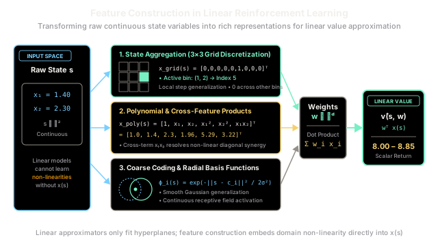
Linear reinforcement learning algorithms can only compute flat hyperplanes over their inputs. Feature construction transforms raw continuous state variables into rich, non-linear representation vectors, enabling linear models to learn complex, curved value functions.
Why Does This Exist?
In reinforcement learning with function approximation, linear methods represent state values as a simple inner product between a learned parameter vector and a feature vector :
Linear function approximators offer decisive mathematical advantages: they are computationally lightweight ( per step), possess a unimodal error surface free from deceptive local minima, and enjoy rigorous convergence guarantees under on-policy Temporal Difference Learning.
However, linear models suffer from a fundamental geometric limitation: they can only fit flat hyperplanes over their input features.
If an agent directly passes raw physical state variables—such as a robot's joint angle and angular velocity —as features , the model can only express values that vary linearly along those axes: . If the true optimal value function is curved, possesses saddle points, or features sharp cliff boundaries (as in Mountain Car or CartPole), a flat hyperplane fails catastrophically. The agent cannot capture multi-variable interactions or localized non-linearities.
Feature construction exists to overcome this representational bottleneck without sacrificing the stability and convergence proofs of linear learning.
By designing non-linear feature mappings —such as state aggregation, polynomial cross-terms, Fourier bases, or radial basis functions—all non-linear complexity is embedded directly into the feature space. The learning algorithm remains strictly linear in its parameter weights , but the composite function can approximate arbitrary, complex non-linear value surfaces.
Think of It Like This
Whole Raw Spices vs. Artisan Spice Blends
Imagine cooking in a commercial kitchen with an automated seasoning dispenser. The machine only has volume dials for its ingredient hoppers; it can adjust how many grams of a powder to pour into a pan, but it cannot chop, roast, grind, or chemically alter ingredients during cooking.
If you dump whole, raw ingredients into the hoppers—unroasted cumin seeds, whole peppercorns, and rock salt crystals (raw continuous state coordinates)—the resulting dish is uneven and bitter. The simple dispenser has no mechanism to crush the seeds or activate aromatic oils. It can only adjust the overall volume of whole seeds.
A master chef solves this through feature engineering (spice preparation):
- Before loading the dispenser, the chef toasts the cumin, grinds the peppercorns, and blends them with smoked paprika and garlic powder into an artisan spice rub (the non-linear feature map ).
- The complex chemical reactions, roasting, and interaction flavors are synthesized beforehand during preparation.
- The automated dispenser now only needs to adjust a single linear volume knob (the weight vector ) to produce an award-winning sauce.
The dispenser remains completely linear and predictable, but the pre-blended features allow it to deliver complex, multi-layered flavors.
Where the analogy stops: Spices degrade chemically over time due to oxidation and humidity. In reinforcement learning, mathematical feature mappings are deterministic, static functions that preserve exact numerical precision across millions of episodes.
How It Actually Works
Linear Value Representation and the Feature Construction Spectrum
When value functions are parameterized linearly, the gradient of the predicted value with respect to the parameter vector is simply the feature vector itself:
This identity makes semi-gradient TD updates exceptionally clean and computationally efficient:
where is the step-size learning rate and is the discount factor. Because updates adjust directly along the active feature directions , the design of dictates how learning generalizes across the state space.
The Representation Spectrum
Practitioners construct feature vectors using several distinct mathematical paradigms:
[Pure Tabular] ────────► [State Aggregation] ────────► [Polynomial & RBF] ────────► [Deep Networks]One-Hot Vector Discretized Grid Bins Continuous Basis Envelopes Learned RepresentationsZero Generalization Step-Wise Generalization Smooth Non-Linear Surface Hierarchical Latentsd = |S| d = B₁ × B₂ × ... × B_D d = Multi-Index Combinations Millions of weights- One-Hot Encoding (Exact Tabular): Each discrete state corresponds to a unique standard basis vector: Updating state affects only , yielding zero generalization across neighboring states.
- State Aggregation (Grid Bins): Continuous state dimensions are partitioned into discrete intervals. All states falling within a given multi-dimensional bin activate a single binary indicator: States inside the same bin share identical value estimates, producing a piecewise-constant step-function approximation.
- Polynomial & Interaction Features: Expands continuous coordinates into products of powers: The cross-term is critical: it allows the model to capture non-linear diagonal synergies where the effect of coordinate depends directly on the magnitude of .
- Fourier Basis: Constructs features using multidimensional cosine waves: where is an integer coefficient vector. Fourier bases provide global, smooth periodic features that excel in continuous kinematic control tasks.
- Radial Basis Functions (RBFs): Defines continuous bell-shaped receptive fields centered at prototype points : Yields smooth, continuous generalization across distance metrics in Euclidean space.
The Generalization vs. Discrimination Trade-Off
The shape and width of constructed feature envelopes govern an inescapable trade-off:
- Broad Feature Envelopes (Large or Large Grid Bins): High generalization. An update at state influences a wide region of neighboring states, speeding up initial learning. However, discrimination is low: the agent cannot resolve fine localized value differences or sharp optimal decision boundaries.
- Narrow Feature Envelopes (Small or Fine Grid Bins): High discrimination. The agent can represent sharp cliffs and localized reward spikes. However, generalization is low: the agent must visit nearly every localized sub-region independently, degrading toward tabular sample complexity.
Worked numerical calculation
Consider an agent navigating a 2D continuous state space , where and .
We evaluate state under two distinct feature construction regimes.
Regime 1: State Aggregation Grid
Each dimension is partitioned into equal intervals of width :
- Coordinate row index .
- Coordinate column index .
The 2D bin coordinate is . Flattening to a 9-dimensional index ():
The resulting constructed feature vector is:
Suppose the learned linear weight vector across the 9 bins is:
The estimated state value is:
Any other state within the bounding box (e.g., ) evaluates to exactly .
Regime 2: Polynomial Expansion with Cross-Product Term
To capture smooth continuous variation and interaction, we construct a 6-dimensional polynomial feature map:
Evaluating each feature term at :
- Bias term:
- Linear terms: ,
- Quadratic terms: ,
- Cross-product interaction term:
The constructed feature vector is:
Let the parameter weights be .
The estimated value is:
Notice that the cross-product interaction term contributed (nearly of the total value). Without feature construction, a purely additive linear model would be blind to this synergistic interaction.
Code
from typing import Dict, List, Tuple
class StateAggregationTransformer: """Discretizes a multi-dimensional continuous state space into a multi-bin grid."""
def __init__( self, bounds: List[Tuple[float, float]], num_bins: List[int], ) -> None: """Initialize discretization intervals.
Args: bounds: List of (min_val, max_val) for each dimension. num_bins: Number of equal-width bins along each dimension. """ assert len(bounds) == len(num_bins), "Bounds and bin counts must match." self.bounds = bounds self.num_bins = num_bins self.total_features = 1 for b in num_bins: self.total_features *= b
def get_bin_indices(self, state: List[float]) -> List[int]: """Convert continuous coordinates into discrete bin indices.""" bin_coords: List[int] = [] for val, (low, high), bins in zip(state, self.bounds, self.num_bins): clamped = max(low, min(high, val)) frac = (clamped - low) / (high - low) bin_idx = min(bins - 1, int(frac * bins)) bin_coords.append(bin_idx) return bin_coords
def transform(self, state: List[float]) -> Dict[int, float]: """Map continuous state to a sparse 1-hot feature dictionary.""" bin_coords = self.get_bin_indices(state) # Convert multi-dimensional coordinate to flat index flat_idx = 0 multiplier = 1 for coord, bins in reversed(list(zip(bin_coords, self.num_bins))): flat_idx += coord * multiplier multiplier *= bins return {flat_idx: 1.0}
def evaluate(self, state: List[float], weights: List[float]) -> float: """Compute linear value estimate v_hat(s, w) = w^T x(s).""" sparse_x = self.transform(state) return sum(weights[idx] * val for idx, val in sparse_x.items())
def polynomial_feature_transform(state: List[float]) -> List[float]: """Expand a 2D continuous state [x1, x2] into quadratic polynomial features.""" assert len(state) == 2, "Expected 2D input state." x1, x2 = state[0], state[1] return [1.0, x1, x2, x1 ** 2, x2 ** 2, x1 * x2]
# Verification matching the worked numerical exampletransformer = StateAggregationTransformer( bounds=[(0.0, 3.0), (0.0, 3.0)], num_bins=[3, 3],)
sample_state = [1.4, 2.3]bin_coords = transformer.get_bin_indices(sample_state)sparse_feat = transformer.transform(sample_state)
assert bin_coords == [1, 2]assert sparse_feat == {5: 1.0}
grid_weights = [1.2, 2.5, 4.0, 2.0, 5.5, 8.0, 3.5, 7.0, 10.0]grid_val = transformer.evaluate(sample_state, grid_weights)assert abs(grid_val - 8.00) < 1e-4
poly_feat = polynomial_feature_transform(sample_state)assert poly_feat == [1.0, 1.4, 2.3, 1.96, 5.29, 3.22]
poly_weights = [0.5, 1.0, 1.5, 0.2, 0.1, 0.8]poly_val = sum(f * w for f, w in zip(poly_feat, poly_weights))assert abs(poly_val - 8.8470) < 1e-4
print(f"State Aggregation Bin: {bin_coords} -> Flat Index: {list(sparse_feat.keys())[0]}")print(f"Grid Discretization Value: {grid_val:.2f}")print(f"Polynomial Features: {poly_feat}")print(f"Polynomial Estimated Value: {poly_val:.4f}")
# -> State Aggregation Bin: [1, 2] -> Flat Index: 5# -> Grid Discretization Value: 8.00# -> Polynomial Features: [1.0, 1.4, 2.3, 1.96, 5.29, 3.22]# -> Polynomial Estimated Value: 8.8470Watch Out For
The Exponential Grid Explosion and Missing Interaction Terms
Two prevalent pitfalls trap engineers when designing linear representations for reinforcement learning:
1. The Curse of Dimensionality in Grid Discretization: Attempting to achieve fine discrimination by dividing every dimension into bins triggers an exponential parameter explosion:
In a 6-DoF robotic manipulator state space ( joint angles and velocities), partitioning each variable into just bins generates features. The memory requirement exceeds terabytes, and sample complexity collapses because each bin must be visited independently to learn its weight.
2. Missing Diagonal Interactions (The Additive Trap): Encoding each state variable with independent 1D features (e.g., ) reduces feature count from to . However, an additive model cannot represent multi-variable interactions. If success requires both and simultaneously (a diagonal decision boundary), purely additive features fail to separate the classes.
Concrete Fix:
- Transition from Grid Discretization to Tile Coding: Tile coding uses multiple overlapping, coarsely quantized tilings with relative offsets. It achieves fine resolution while scaling linearly with the number of tilings rather than exponentially with resolution.
- Include Multi-Variable Cross Products: Always augment independent 1D basis functions with pairwise interaction terms (such as or conjunctive tile intersections) whenever physical variables exhibit dynamic coupling.
The Quick Version
- Linear value approximators can only fit hyperplanes; feature construction embeds all non-linear domain complexity directly into .
- Feature design controls the generalization-discrimination trade-off: broad features generalize quickly, while narrow features resolve sharp boundaries.
- Constructing interaction terms (e.g., or conjunctive receptive fields) is essential to capture diagonal synergies that purely additive models cannot express.
- Naive multi-dimensional grid discretization explodes exponentially (), necessitating advanced sparse representations like tile coding or Fourier bases in higher dimensions.