Tile Coding (CMAC) in RL
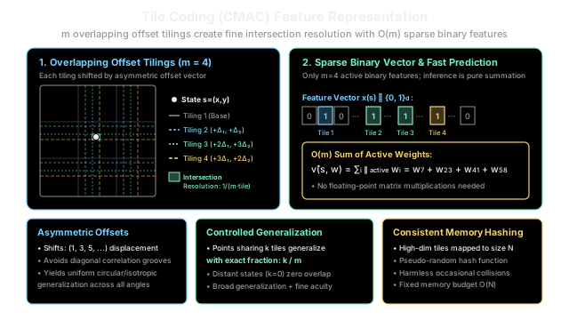
Tile coding overlays multiple slightly shifted grid patterns across continuous space, translating coordinates into a sparse set of active tiles that combine broad generalization with pinpoint resolution.
Why Does This Exist?
When reinforcement learning agents operate in continuous state spaces—such as a robotic arm moving through 3D coordinates or a self-balancing cart-pole—tabular methods fail because no continuous state is ever visited twice.
A naive workaround is to discretize the state space into a single coarse grid. However, a single grid suffers from two critical flaws:
- Severe quantization error: All continuous points within the same grid cell are treated as identical, producing stair-step, piecewise-constant value functions with harsh discontinuities at cell borders.
- The curse of resolution vs. generalization: If cells are large, the agent cannot make fine-grained control distinctions; if cells are tiny, memory requirements explode exponentially () and learning generalizes virtually zero distance.
Introduced by James Albus in 1975 under the name CMAC (Cerebellar Model Articulation Controller) and popularized in reinforcement learning by Richard Sutton, tile coding elegantly resolves this trade-off. By superimposing multiple overlapping grid partitions (tilings) shifted by small asymmetric offsets, the intersection of active tiles achieves high spatial resolution while retaining the broad, smooth generalization of large tiles—all while producing sparse binary feature vectors that compute in integer time.
Think of It Like This
The Draftsman's Offset Grid Stencils
Imagine an artist trying to identify the precise coordinates of a pinhole on a drafting canvas using grid stencils:
- A Single Coarse Stencil: She lays down one stencil with 2-inch square cutouts. The pinhole falls into cell
(row 3, col 2). This tells her the pinhole's general neighborhood, but she has zero idea whether it is sitting near the top-left or bottom-right corner of that 2-inch box. - Multiple Offset Stencils (Tile Coding): Instead of making the stencil squares microscopic (which would require millions of tiny cutouts), she lays down four identical stencils, each shifted slightly in a different direction:
- Stencil 1 is aligned at the canvas origin.
- Stencil 2 is nudged half an inch right and a quarter inch down.
- Stencil 3 is nudged an inch right and three-quarters down.
- Stencil 4 is nudged an inch and a half right and half an inch down.
Now, she marks which box contains the pinhole on each of the four sheets. When all four stencils are stacked together, the overlapping intersection of the four marked boxes forms a tiny sub-box just a fraction of an inch wide!
Where the analogy stops: Real drafting stencils physically occlude light. In tile coding, the active tiles are represented digitally as indices in a sparse binary feature vector , where exactly one feature per tiling equals and all others are .
How It Actually Works
Overlapping Tilings and Asymmetric Offsets
Let the continuous state space be . A tiling is an exhaustive partitioning of the state space into non-overlapping geometric hyper-rectangles called tiles.
Tile coding uses distinct tilings. Each tiling has identical tile dimensions (width along dimension ), but each tiling is displaced relative to the others by an offset vector :
For any continuous state , the integer coordinate of the active tile in tiling along dimension is calculated via floor division:
To prevent unnatural diagonal alignment artifacts, offsets must be chosen asymmetrically. If tilings are shifted uniformly along diagonals (), the intersections form diagonal elongated strips, causing the value function to generalize unnaturally along the 45-degree axis. Sutton and Barto recommend displacing tilings using odd-integer displacement vectors:
This asymmetric spacing ensures that the overlapping intersection regions are nearly isotropic (square/circular), providing balanced generalization across all spatial directions.
Sparsity and O(m) Computational Efficiency
Because each tiling is an exhaustive partition, any continuous state falls into exactly one tile per tiling. For a system with tilings:
- The binary feature vector contains millions of possible tile dimensions.
- However, exactly features are non-zero ( and ).
- All remaining features are strictly .
This extreme sparsity transforms linear value inference from an expensive vector multiplication into a fast integer lookup:
Rather than executing floating-point multiplications, computing requires only memory lookups and additions ( complexity), completely independent of total state-space resolution .
Proportional Generalization and Tile Hashing
-
Controlled Generalization: Two continuous states and generalize in direct proportion to their spatial proximity. If and share active tiles across the tilings, their feature dot product is: Updating state shifts the value of state by exactly the fraction . Points separated by more than one tile width share zero tiles () and undergo zero cross-talk.
-
Consistent Tile Hashing: In multi-dimensional spaces, the total number of tiles across all tilings can easily reach billions. To cap memory usage, multi-dimensional tile coordinates are mapped to a fixed-size weight table of length using a uniform pseudo-random hash function: Because tilings are offset and states are sparse, occasional hash collisions are spread uniformly throughout the state space, behaving as harmless pseudo-random noise that averages out during learning.
Worked numerical calculation
Consider a 2-dimensional continuous state .
- Number of tilings: .
- Tile width along both axes: .
- Fundamental offset step: .
- Asymmetric offsets for the 4 tilings:
- Tiling 0:
- Tiling 1:
- Tiling 2:
- Tiling 3:
Compute active tile integer coordinates :
-
Tiling 0: Active Tile:
(Tiling 0, Tile [1, 3]) -
Tiling 1: Active Tile:
(Tiling 1, Tile [1, 2]) -
Tiling 2: Active Tile:
(Tiling 2, Tile [1, 3]) -
Tiling 3: Active Tile:
(Tiling 3, Tile [1, 3])
Suppose the current learned weights associated with these four active tiles are:
The estimated linear state value is the direct sum of the active weights:
Computing this prediction required exactly four additions, delivering high-acuity localization with minimal processor overhead.
Code
import mathfrom typing import Dict, List, Set, Tuple
class TileCoder2D: """2D Tile Coder (CMAC) using asymmetric offsets and linear weight indexing."""
def __init__( self, num_tilings: int = 4, tile_width: float = 2.0, offsets: List[Tuple[float, float]] = None, ): self.num_tilings = num_tilings self.tile_width = tile_width
# Asymmetric offsets to prevent diagonal correlation artifacts if offsets is None: self.offsets = [ (0.0, 0.0), (0.5, 1.5), (1.0, 1.0), (1.5, 0.5), ] else: assert len(offsets) == num_tilings self.offsets = offsets
def get_active_tiles(self, x: float, y: float) -> List[Tuple[int, int, int]]: """Return the active (tiling_idx, coord_x, coord_y) for continuous point (x, y).""" active_tiles: List[Tuple[int, int, int]] = [] for tiling_idx, (ox, oy) in enumerate(self.offsets): cx = math.floor((x - ox) / self.tile_width) cy = math.floor((y - oy) / self.tile_width) active_tiles.append((tiling_idx, cx, cy)) return active_tiles
def predict( self, x: float, y: float, weights: Dict[Tuple[int, int, int], float] ) -> float: """Compute linear prediction as sum of m active tile weights in O(m) time.""" active_tiles = self.get_active_tiles(x, y) return sum(weights.get(tile, 0.0) for tile in active_tiles)
def update( self, x: float, y: float, target: float, weights: Dict[Tuple[int, int, int], float], alpha: float = 0.1, ) -> float: """Perform linear semi-gradient update: w_i <- w_i + (alpha / m) * (target - v_hat).""" active_tiles = self.get_active_tiles(x, y) v_hat = sum(weights.get(tile, 0.0) for tile in active_tiles) error = target - v_hat
# Step size normalized by number of active tilings m step_size = alpha / self.num_tilings for tile in active_tiles: weights[tile] = weights.get(tile, 0.0) + step_size * error
return error
if __name__ == "__main__": tc = TileCoder2D(num_tilings=4, tile_width=2.0) query_x, query_y = 3.6, 7.2
# 1. Active Tile Indexing Verification active = tc.get_active_tiles(query_x, query_y) print("=== Tile Coding (CMAC) Numerical Verification ===") print(f"Continuous State Point: ({query_x}, {query_y})") print(f"Active Tile Indices across {tc.num_tilings} tilings:") for tile in active: print(f" Tiling {tile[0]}: Tile Coordinate [{tile[1]}, {tile[2]}]")
expected_active = [(0, 1, 3), (1, 1, 2), (2, 1, 3), (3, 1, 3)] assert ( active == expected_active ), f"Expected {expected_active}, got {active}"
# 2. Value Prediction Verification with Preset Weights preset_weights: Dict[Tuple[int, int, int], float] = { (0, 1, 3): 1.20, (1, 1, 2): 0.80, (2, 1, 3): 1.50, (3, 1, 3): 1.00, } v_val = tc.predict(query_x, query_y, preset_weights) print(f"\nCalculated Linear Value v_hat: {v_val:.2f}") assert math.isclose(v_val, 4.50), f"Expected 4.50, got {v_val}"
# 3. Spatial Generalization Verification close_point = (3.7, 7.3) far_point = (6.5, 11.0)
set_original: Set[Tuple[int, int, int]] = set(active) set_close: Set[Tuple[int, int, int]] = set( tc.get_active_tiles(*close_point) ) set_far: Set[Tuple[int, int, int]] = set(tc.get_active_tiles(*far_point))
overlap_close = len(set_original.intersection(set_close)) overlap_far = len(set_original.intersection(set_far))
print("\nGeneralization Analysis:") print( f" Nearby point {close_point} shares: {overlap_close}/4 tiles ({overlap_close / 4:.0%} overlap)" ) print( f" Distant point {far_point} shares: {overlap_far}/4 tiles ({overlap_far / 4:.0%} overlap)" )
assert ( overlap_close >= 3 ), "Close continuous points must share significant tile overlap!" assert ( overlap_far == 0 ), "Far continuous points must share zero tile overlap!"
print("\nAll tile coding mathematical assertions passed successfully.")
# Expected Output:# === Tile Coding (CMAC) Numerical Verification ===# Continuous State Point: (3.6, 7.2)# Active Tile Indices across 4 tilings:# Tiling 0: Tile Coordinate [1, 3]# Tiling 1: Tile Coordinate [1, 2]# Tiling 2: Tile Coordinate [1, 3]# Tiling 3: Tile Coordinate [1, 3]## Calculated Linear Value v_hat: 4.50## Generalization Analysis:# Nearby point (3.7, 7.3) shares: 4/4 tiles (100% overlap)# Distant point (6.5, 11.0) shares: 0/4 tiles (0% overlap)## All tile coding mathematical assertions passed successfully.Watch Out For
Symmetrical Offsets and Diagonal Bias Grooves
A frequent pitfall when building custom tile coders is choosing uniform symmetrical tiling offsets, such as shifting each successive tiling by equal increments along every axis:
When offsets are symmetrical:
- The sub-tile intersection shapes elongate into narrow diagonal slivers oriented along the 45-degree axis.
- The agent generalizes strongly along the diagonal while generalizing poorly along orthogonal directions.
- Learning develops artificial "grooves," causing erratic policy performance when negotiating curved trajectories.
The Fix:
- Use Odd-Integer Asymmetric Vectors: Follow the canonical Sutton-Barto offset construction where coordinate displacements follow , creating isotropic, nearly circular receptive fields.
- Dimension-Specific Tile Widths: Tune tile widths independently per dimension to reflect physical sensitivity (e.g., narrow tiles for sensitive angle sensors and wide tiles for cart position).
- Choose Tilings: Using too few tilings () causes coarse stair-step value approximations; using yields smooth, quasi-continuous function approximation.
The Quick Version
- Multiple offset grids: Tile coding overlays complete partitionings (tilings) of continuous state space, displaced by asymmetric offsets.
- Sparse binary representation: Exactly tiles are active at any continuous point; the feature vector is purely binary with .
- Lightning-fast inference: Value estimation evaluates as a simple sum of active weights, completely bypassing matrix multiplications.
- Isotropic generalization: Two states sharing active tiles generalize with exact weight fraction , combining broad coverage with pinpoint spatial resolution.