Radial Basis Functions in RL

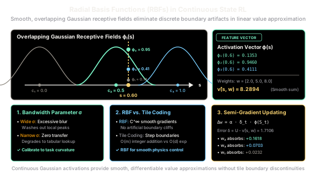
Unlike grid discretization or tile coding that divide space with sharp binary edges, radial basis functions produce smooth, bell-shaped receptive fields. Each continuous state activates neighboring basis centers in proportion to its distance, yielding continuously differentiable value surfaces.

Radial basis functions produce smooth, continuous Gaussian activations centered at prototype coordinates, enabling linear value approximators to learn differentiable value surfaces without step-boundary artifacts.

Why Does This Exist?

In continuous control problems—such as balancing an inverted pendulum, flying an autonomous drone, or navigating a robotic arm—state variables like angle, velocity, and torque vary continuously.

When applying linear function approximation to continuous state spaces, classical representations like state aggregation and Coarse Coding rely on binary membership features: a state either falls inside a discrete tile ( $x_i(s) = 1$ ) or it does not ( $x_i(s) = 0$ ).

This discrete quantization introduces critical problems in gradient-based reinforcement learning:

Discontinuous Step Artifacts: The approximated value function $\hat{v}(s, \mathbf{w})$ resembles a staircase of flat plateaus separated by sharp cliff boundaries. Crossing a tile boundary triggers sudden, jarring jumps in value predictions.
Zero Gradients for Policy Optimization: In actor-critic and policy gradient methods, continuous action selection often relies on the spatial gradient of the value surface $\nabla_s \hat{v}(s, \mathbf{w})$ . On flat plateaus, the spatial gradient is identically zero ( $\nabla_s \hat{v} = \mathbf{0}$ ), providing zero directional guidance to the policy. At boundary edges, the gradient is non-differentiable or infinite.

Radial Basis Functions (RBFs) exist to provide smooth, continuous, and infinitely differentiable ( $C^\infty$ ) feature representations.

Instead of hard binary partitions, RBFs deploy continuous bell-shaped receptive fields—most commonly Gaussian curves—centered at prototype coordinates across the state space. As an agent moves continuously through the environment, its feature activations shift smoothly between zero and one. This eliminates artificial boundary cliffs, enables analytical spatial gradients $\nabla_s \hat{v}(s, \mathbf{w})$ , and allows linear models to represent curved, organic value surfaces.

Think of It Like This

The Diffuse Theater Spotlights

Imagine walking across a dark theater stage illuminated by overhead spotlights aimed at three distinct floor positions: stage left ( $c_1 = 0.0$ ), center stage ( $c_2 = 0.5$ ), and stage right ( $c_3 = 1.0$ ).

These are not theatrical profile spots with sharp, knife-edge shutters that cast crisp geometric squares on the floor (which would be tile coding). Instead, each light is fitted with a soft diffusion frost lens. At the exact center of a spotlight's beam, the illumination is at peak brightness ( $100\%$ ). As you move away from the center, the brightness tapers off smoothly in all directions following a Gaussian bell curve.

Suppose you stand at coordinate $s = 0.60$ (slightly to the right of center stage):

Center Stage Spotlight ( $c_2 = 0.50$ ) is only $0.10$ meters away: its beam strikes you with strong, direct illumination at $95\%$ intensity ( $\phi_2 = 0.95$ ).
Stage Right Spotlight ( $c_3 = 1.00$ ) is $0.40$ meters away: its peripheral halo casts a moderate $41\%$ illumination on you ( $\phi_3 = 0.41$ ).
Stage Left Spotlight ( $c_1 = 0.00$ ) is far away across the stage: its ambient fringe reaches you at a faint $14\%$ glow ( $\phi_1 = 0.14$ ).

Your overall visibility is the weighted sum of all three overlapping light beams. As you take a step, your lighting does not flicker, strobe, or jump abruptly across an invisible border. The light transitions seamlessly from one beam to the next.

Where the analogy stops: In optics, light beams combine strictly via positive physical superposition (you cannot project "negative light"). In reinforcement learning, RBF linear weights $w_i$ can be negative, allowing the learned value surface to represent deep negative penalty valleys and sharp reward peaks with equal fluidity.

How It Actually Works

Gaussian RBF Formulation, Bandwidth Tuning, and Semi-Gradient Updates

In an RBF network, a continuous state $s \in \mathbb{R}^D$ is transformed into a $d$ -dimensional continuous feature vector $\boldsymbol{\phi}(s) = [\phi_1(s), \dots, \phi_d(s)]^\top$ .

The Gaussian Basis Function

The standard Gaussian radial basis function $\phi_i(s)$ is parameterized by a prototype center coordinate $\mathbf{c}_i \in \mathbb{R}^D$ and a bandwidth standard deviation $\sigma_i > 0$ :

\phi_i(s) \doteq \exp\left( -\frac{\|s - \mathbf{c}_i\|^2}{2\sigma_i^2} \right)

where:

$\|s - \mathbf{c}_i\|$ is the Euclidean distance between state $s$ and basis center $\mathbf{c}_i$ .
$\phi_i(s) \in (0, 1]$ represents the degree of membership or activation.
When $s = \mathbf{c}_i$ , the exponent evaluates to zero, yielding maximal activation $\phi_i(\mathbf{c}_i) = 1.0$ .
As distance $\|s - \mathbf{c}_i\| \to \infty$ , activation decays exponentially toward zero.

For multi-dimensional spaces where dimensions have different physical units (e.g., position vs. velocity), each basis can use a diagonal covariance matrix $\boldsymbol{\Sigma}_i = \text{diag}(\sigma_{i,1}^2, \dots, \sigma_{i,D}^2)$ :

\phi_i(s) = \exp\left( -\frac{1}{2} \sum_{k=1}^D \frac{(s_k - c_{i,k})^2}{\sigma_{i,k}^2} \right)

Linear Value Approximation and Spatial Gradients

The state-value estimate $\hat{v}(s, \mathbf{w})$ is the linear combination of basis activations and learned weights $\mathbf{w} \in \mathbb{R}^d$ :

\hat{v}(s, \mathbf{w}) \doteq \mathbf{w}^\top \boldsymbol{\phi}(s) = \sum_{i=1}^d w_i \phi_i(s)

Because the Gaussian exponential is smooth and infinitely differentiable, the spatial gradient with respect to the state coordinates $s$ is analytically available:

\nabla_s \hat{v}(s, \mathbf{w}) = \sum_{i=1}^d w_i \phi_i(s) \left( -\frac{s - \mathbf{c}_i}{\sigma_i^2} \right)

This analytical gradient allows continuous actor-critic algorithms to perform policy optimization directly via backpropagation into action parameters.

Semi-Gradient TD Update Rule

Under semi-gradient Temporal Difference Learning, observing transition $(S_t, R_{t+1}, S_{t+1})$ produces scalar TD error:

\delta_t = R_{t+1} + \gamma \hat{v}(S_{t+1}, \mathbf{w}_t) - \hat{v}(S_t, \mathbf{w}_t)

Weights are updated in the direction of the basis gradient $\nabla_\mathbf{w} \hat{v}(S_t, \mathbf{w}) = \boldsymbol{\phi}(S_t)$ :

\mathbf{w}_{t+1} = \mathbf{w}_t + \alpha \delta_t \boldsymbol{\phi}(S_t)

where $\alpha \in (0, 1]$ is the step size. Crucially, every weight $w_i$ is updated in direct proportion to its active participation $\phi_i(S_t)$ in the visited state.

Bandwidth Tuning: The Over-smoothing vs. Dead-Zone Dilemma

The bandwidth parameter $\sigma$ governs the spatial width of generalization:

1Receptive Field Envelopes2       Wide σ (Oversmoothing)          Optimal σ (Smooth Overlap)          Narrow σ (Dead Zones)3   ┌────────────────────────────┐    ┌────────────────────────────┐    ┌────────────────────────────┐4   │          ╭──────╮          │    │      ╭──╮        ╭──╮      │    │     ││            ││       │5   │      ╭───╯      ╰───╮      │    │    ╭─╯  ╰─╮    ╭─╯  ╰─╮    │    │    ╭╯╰╮          ╭╯╰╮      │6   │  ────╯              ╰────  │    │  ──╯      ╰────╯      ╰──  │    │  ──╯  ╰──────────╯  ╰──    │7   └────────────────────────────┘    └────────────────────────────┘    └────────────────────────────┘8     Washes out sharp peaks            Balanced generalization           Zero transfer, gap artifacts

Wide $\sigma$ (Excessive Overlap): Value updates generalize over wide regions of state space. However, localized reward peaks and fine decision boundaries are blurred into a featureless average.
Narrow $\sigma$ (Insufficient Overlap): Receptive fields barely touch. In regions between prototype centers, all basis activations drop to near zero ( $\boldsymbol{\phi}(s) \approx \mathbf{0}$ ). These "dead zones" cause predictions to collapse to zero and freeze learning gradients.
Calibrated Rule of Thumb: Set $\sigma$ approximately equal to the spacing between adjacent centers ( $\sigma \approx \Delta c$ ) so that adjacent basis functions intersect at roughly $\phi \approx 0.50$ to $0.60$ .

RBFs vs. Tile Coding

Feature Attribute	Gaussian RBFs	Tile Coding
Surface Smoothness	$C^\infty$ continuously differentiable	Piecewise-constant step function
Boundary Artifacts	Zero boundary discontinuities	Step-edge artifacts at tile borders
Compute Complexity	$O(d \cdot D)$ transcendental exponentials	$O(m)$ sparse integer additions
Sparsity	Dense (all bases active to some degree)	Strictly sparse (exactly $m$ active tiles)
High Dimensions	Suffers severe curse of dimensionality	Scalable via hashing and sparse tilings

Worked numerical calculation

Consider an agent navigating a 1D continuous state space $s \in [0.0, 1.0]$ .

We configure a 3-basis Gaussian RBF network:

Centers: $c_1 = 0.0, c_2 = 0.5, c_3 = 1.0$
Uniform bandwidth: $\sigma = 0.3$
Denominator: $2\sigma^2 = 2(0.3)^2 = 2(0.09) = \mathbf{0.18}$
Initial weight vector: $\mathbf{w} = [2.0000, 5.0000, 8.0000]^\top$
Step-size parameter: $\alpha = 0.1$

We evaluate the continuous state $s = 0.60$ and apply a semi-gradient update with observed target return $U = 10.0$ .

Step 1: Compute Basis Feature Activations $\boldsymbol{\phi}(0.60)$

Basis 1 ( $c_1 = 0.0$ ): $(0.60 - 0.0)^2 = 0.3600 \implies \phi_1(0.60) = \exp\left(-\frac{0.3600}{0.18}\right) = \exp(-2.0000) = \mathbf{0.1353}$
Basis 2 ( $c_2 = 0.5$ ): $(0.60 - 0.5)^2 = 0.0100 \implies \phi_2(0.60) = \exp\left(-\frac{0.0100}{0.18}\right) = \exp(-0.0556) = \mathbf{0.9460}$
Basis 3 ( $c_3 = 1.0$ ): $(0.60 - 1.0)^2 = 0.1600 \implies \phi_3(0.60) = \exp\left(-\frac{0.1600}{0.18}\right) = \exp(-0.8889) = \mathbf{0.4111}$

The constructed feature vector is:

\boldsymbol{\phi}(0.60) = [0.1353, 0.9460, 0.4111]^\top

Step 2: Compute Predicted Value $\hat{v}(0.60, \mathbf{w})$

Taking the inner product $\mathbf{w}^\top \boldsymbol{\phi}(0.60)$ :

\begin{aligned} \hat{v}(0.60, \mathbf{w}) &= w_1 \phi_1 + w_2 \phi_2 + w_3 \phi_3 \\ &= 2.0000(0.135335) + 5.0000(0.945959) + 8.0000(0.411112) \\ &= 0.2707 + 4.7298 + 3.2889 \\ &= \mathbf{8.2894} \end{aligned}

Step 3: Compute Prediction Error and Weight Updates

With target return $U = 10.0$ :

\delta = U - \hat{v}(0.60, \mathbf{w}) = 10.0000 - 8.2894 = \mathbf{1.7106}

Applying the update $\mathbf{w} \leftarrow \mathbf{w} + \alpha \delta \boldsymbol{\phi}(0.60)$ with $\alpha = 0.1$ :

Weight 1 ( $c_1 = 0.0$ ): $\Delta w_1 = 0.1 \times 1.7106 \times 0.135335 = +0.0232 \implies w_1 \leftarrow 2.0000 + 0.0232 = \mathbf{2.0232}$
Weight 2 ( $c_2 = 0.5$ ): $\Delta w_2 = 0.1 \times 1.7106 \times 0.945959 = +0.1618 \implies w_2 \leftarrow 5.0000 + 0.1618 = \mathbf{5.1618}$
Weight 3 ( $c_3 = 1.0$ ): $\Delta w_3 = 0.1 \times 1.7106 \times 0.411112 = +0.0703 \implies w_3 \leftarrow 8.0000 + 0.0703 = \mathbf{8.0703}$

Notice that Center 2 absorbs $63\%$ of the total update ( $\Delta w_2 = 0.1618$ ) because it is nearest to $s=0.60$ , while neighboring centers smoothly receive proportional fractional updates without boundary truncation.

Code

1import math2from typing import List, Optional, Tuple3
4
5class GaussianRBFValueApproximator:6    """Linear value function approximator using continuous Gaussian Radial Basis Functions."""7
8    def __init__(9        self,10        centers: List[float],11        sigma: float,12        initial_weights: Optional[List[float]] = None,13    ) -> None:14        """Initialize RBF network.15
16        Args:17            centers: List of 1D center prototype coordinates c_i.18            sigma: Standard deviation / bandwidth parameter for all bases.19            initial_weights: Optional initial weight vector w.20        """21        self.centers = centers22        self.sigma = sigma23        self.denom = 2.0 * (sigma ** 2)24        self.num_bases = len(centers)25        self.weights = (26            initial_weights.copy()27            if initial_weights is not None28            else [0.0] * self.num_bases29        )30
31    def compute_features(self, state: float) -> List[float]:32        """Compute continuous Gaussian RBF feature vector phi(s) in (0, 1]^d.33
34        Args:35            state: Continuous 1D state coordinate s.36
37        Returns:38            Vector of basis activations [phi_1(s), ..., phi_d(s)].39        """40        return [41            math.exp(-((state - c) ** 2) / self.denom)42            for c in self.centers43        ]44
45    def predict(self, state: float) -> float:46        """Evaluate estimated state value v_hat(s, w) = w^T phi(s)."""47        features = self.compute_features(state)48        return sum(w * phi for w, phi in zip(self.weights, features))49
50    def update(51        self,52        state: float,53        target_value: float,54        alpha: float = 0.1,55    ) -> Tuple[float, List[float]]:56        """Perform a semi-gradient TD / Monte Carlo update step.57
58        Args:59            state: Continuous state s where update target was observed.60            target_value: Sample return or TD target U_t.61            alpha: Step-size learning rate.62
63        Returns:64            Tuple of (prediction_error delta, updated_weight_vector).65        """66        features = self.compute_features(state)67        prediction = sum(w * phi for w, phi in zip(self.weights, features))68        delta = target_value - prediction69
70        for i in range(self.num_bases):71            self.weights[i] += alpha * delta * features[i]72
73        return delta, self.weights.copy()74
75
76# Verification matching the worked numerical calculation77rbf_model = GaussianRBFValueApproximator(78    centers=[0.0, 0.5, 1.0],79    sigma=0.3,80    initial_weights=[2.0, 5.0, 8.0],81)82
83test_state = 0.6084features = rbf_model.compute_features(test_state)85
86assert abs(features[0] - 0.1353) < 1e-487assert abs(features[1] - 0.9460) < 1e-488assert abs(features[2] - 0.4111) < 1e-489
90initial_val = rbf_model.predict(test_state)91assert abs(initial_val - 8.2894) < 1e-492
93# Execute semi-gradient update with target return U = 10.0 and alpha = 0.194err, new_w = rbf_model.update(state=test_state, target_value=10.0, alpha=0.1)95
96assert abs(err - 1.7106) < 1e-497assert abs(new_w[0] - 2.0232) < 1e-498assert abs(new_w[1] - 5.1618) < 1e-499assert abs(new_w[2] - 8.0703) < 1e-4100
101print(f"RBF Features at s={test_state}: {[round(f, 4) for f in features]}")102print(f"Predicted Value v_hat(s): {initial_val:.4f}")103print(f"Prediction Error delta: {err:.4f}")104print(f"Updated Weights w: {[round(w, 4) for w in new_w]}")105
106# -> RBF Features at s=0.6: [0.1353, 0.946, 0.4111]107# -> Predicted Value v_hat(s): 8.2894108# -> Prediction Error delta: 1.7106109# -> Updated Weights w: [2.0232, 5.1618, 8.0703]

Watch Out For

The Exponential Basis Scaling Curse and Unnormalized Dead Zones

Deploying RBF networks in multi-dimensional reinforcement learning introduces two severe failure modes:

1. Dimensionality Explosion and Computational Bottlenecks: Placing RBF centers on a regular grid across $D$ continuous dimensions requires $K^D$ basis functions. For an 8-dimensional robot arm with $K = 5$ centers per dimension, the network requires $5^8 = 390,625$ centers. Unlike Tile Coding, where only a sparse handful ( $m \approx 16$ ) of tiles are active per step, RBFs are dense: every single update evaluates $O(d \cdot D)$ Euclidean distances and exponential transcendental functions, collapsing training throughput.

2. Unnormalized Dead Zones: If centers are placed too far apart relative to bandwidth $\sigma$ , regions between prototypes have near-zero activations ( $\sum_i \phi_i(s) \ll 1$ ). Value predictions in these dead zones collapse toward zero, and gradients vanish, trapping agents in unlearned regions.

Concrete Fix:

Never use Cartesian grids in high dimensions: Sample RBF centers along actual agent trajectories, or use $k$ -means clustering on replay buffer observations to allocate centers exclusively to reachable regions of state space.
Normalize activations via Normalized RBFs (Softmax Basis): Normalize basis activations so they form a partition of unity summing to $1.0$ : $\tilde{\phi}_i(s) \doteq \frac{\phi_i(s)}{\sum_{j=1}^d \phi_j(s)}$ This eliminates dead zones entirely, ensuring every state receives a well-scaled value estimate and active learning gradient.

The Quick Version

Radial Basis Functions provide continuous, infinitely differentiable Gaussian feature activations for linear reinforcement learning.
By replacing sharp binary memberships with smooth bell curves, RBFs eliminate step-function artifacts and provide analytical spatial gradients $\nabla_s \hat{v}$ .
Bandwidth $\sigma$ governs the generalization trade-off: wide $\sigma$ washes out local value peaks, while narrow $\sigma$ creates unlearned dead zones.
While smooth and expressive in low dimensions, RBFs are computationally denser than tile coding ( $O(d)$ transcendental exponentials vs $O(m)$ sparse additions).