Deep Deterministic Policy Gradient (DDPG)

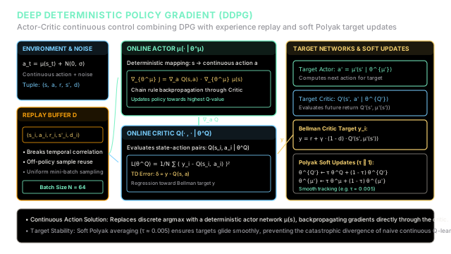
DDPG adapts deep Q-learning to continuous action spaces using an actor network to output exact actions and soft target networks to maintain stable updates.

Why Does This Exist?

In discrete action spaces, Deep Q-Networks (DQN) compute Bellman targets by taking the maximum over all possible actions:

$y = R_{t+1} + \gamma \max_{a' \in \mathcal{A}} Q(S_{t+1}, a')$

When $|\mathcal{A}|$ is small (e.g., 4 or 18 joystick buttons in Atari), this maximization is trivial: the network outputs a scalar for each discrete action, and the agent selects the highest value via an $\arg\max$ operation.

However, in continuous control tasks—such as robotic limb articulation, aerospace navigation, and autonomous driving—actions are real-valued vectors ( $a \in \mathbb{R}^d$ ). Finding $\max_{a'} Q(s', a')$ over a continuous, high-dimensional space requires solving a non-convex global optimization problem at every single time step, which is computationally intractable in deep neural networks. Discretizing each action dimension fails due to the curse of dimensionality: discretizing an 8-joint robotic manipulator into 10 bins per joint creates $10^8 = 100,000,000$ discrete actions, exploding computational cost and discarding the fine-grained precision necessary for physical control.

In 2015, Timothy Lillicrap et al. introduced Deep Deterministic Policy Gradient (DDPG). DDPG bridges the gap between deep Q-learning and continuous control by combining:

The Deterministic Policy Gradient (DPG) theorem (Silver et al., 2014): Instead of searching for the optimal action numerically, an actor network $\mu(s \mid \theta^\mu)$ is trained to directly output the continuous action vector that maximizes the critic's Q-value.
Experience Replay: An off-policy replay buffer $\mathcal{D}$ stores past transitions $(s, a, r, s', d)$ , breaking temporal correlations and enabling sample reuse.
Polyak Soft Target Updates: Rather than copying target network weights periodically (which causes abrupt target shocks), DDPG slowly tracks online parameters via soft averaging ( $\tau \ll 1$ ), ensuring numerical stability.

Think of It Like This

The Formula 1 Driver and the Telemetry Engineer

Imagine an apprentice Formula 1 racing driver coached by a veteran telemetry engineer:

The Actor (The Apprentice Driver $\mu$ ): The driver sits in the cockpit controlling continuous steering wheel angles, brake pressure, and throttle percentages. The driver does not pick from a discrete list of commands—they modulate exact physical inputs in real time.
The Critic (The Telemetry Engineer $Q$ ): The telemetry engineer sits in the pit wall monitoring vehicle dynamics, tyre slip angles, and lap split times. The engineer does not steer the car, but they score the expected lap time for any specific steering angle executed at any specific corner ( $Q(s, a)$ ).

During debriefs, the engineer provides precise gradient guidance to the driver: "Turning the wheel $2^\circ$ sharper at the apex of Turn 3 would have gained $0.15\text{ seconds}$ on exit speed" ( $\nabla_a Q$ ). The driver directly updates their muscle memory in that direction ( $\nabla_{\theta^\mu} \mu$ ), learning to steer precisely where the telemetry predicts the highest return.

Both driver and engineer study past laps recorded on a black-box flight recorder (the replay buffer), ensuring they learn from diverse track conditions without overfitting to the most recent turn.

To prevent an erratic positive feedback loop—where the driver changes their driving style too abruptly, confusing the engineer's calculations, causing the car to spin out—the team uses slow-moving reference blueprints (Polyak target networks). The blueprints adjust by a tiny fraction ( $\tau = 0.5\%$ ) on each lap, guaranteeing that reference targets glide smoothly without destabilizing the vehicle mid-corner.

Where the analogy stops: Telemetry engineers rely on physical aerodynamic and tyre friction equations. In DDPG, the critic has no innate physics knowledge—it learns purely by bootstrapping from scalar environment rewards, meaning early critic approximation errors can misguide the actor toward over-optimistic actions.

How It Actually Works

Deterministic Policy Gradient Theorem and Soft Target Tracking

DDPG maintains four neural networks:

Online Actor $\mu(s \mid \theta^\mu)$ : Maps state $s$ to a continuous action vector $a \in \mathbb{R}^d$ .
Online Critic $Q(s, a \mid \theta^Q)$ : Maps state-action pair $(s, a)$ to a scalar expected return $Q \in \mathbb{R}$ .
Target Actor $\mu'(s \mid \theta^{\mu'})$ : Slowly tracking copy of the actor network.
Target Critic $Q'(s, a \mid \theta^{Q'})$ : Slowly tracking copy of the critic network.

1. Critic Optimization

The critic is trained off-policy using transitions sampled uniformly from the replay buffer $\mathcal{D}$ . For a mini-batch of transitions $(s_i, a_i, r_i, s'_i, d_i)$ , where $d_i \in \{0, 1\}$ indicates whether state $s'_i$ is terminal:

The target value $y_i$ is computed using the target networks:

$y_i = r_i + \gamma (1 - d_i) Q' \left( s'_i, \mu'(s'_i \mid \theta^{\mu'}) \mid \theta^{Q'} \right)$

The critic parameters $\theta^Q$ minimize the mean squared Bellman error:

$\mathcal{L}(\theta^Q) = \frac{1}{N} \sum_{i=1}^N \left( y_i - Q(s_i, a_i \mid \theta^Q) \right)^2$

2. Actor Optimization via Deterministic Policy Gradient

According to the Deterministic Policy Gradient theorem, the objective is to maximize expected performance $J(\theta^\mu) = \mathbb{E}_{s \sim \rho^\beta}[Q(s, \mu(s \mid \theta^\mu))]$ . By applying the chain rule, the gradient of the performance objective with respect to the actor parameters $\theta^\mu$ is:

$\nabla_{\theta^\mu} J \approx \frac{1}{N} \sum_{i=1}^N \left. \nabla_a Q(s_i, a \mid \theta^Q) \right|_{a = \mu(s_i \mid \theta^\mu)} \nabla_{\theta^\mu} \mu(s_i \mid \theta^\mu)$

This formula reveals the elegance of DPG:

$\nabla_a Q(s, a)$ : Measures how the critic's evaluated return changes as the action changes (points in the direction of higher Q-value).
$\nabla_{\theta^\mu} \mu(s)$ : Measures how the actor's network parameters change the action output.
Multiplying them updates the actor in the exact parameter direction that increases the critic's Q-value.

3. Polyak Soft Target Updates

In DQN, target network parameters are held fixed and copied periodically every $C$ steps ( $\theta^- \leftarrow \theta$ ), creating periodic discontinuities in the loss landscape. DDPG replaces this with continuous Polyak averaging (soft updates) performed after every gradient step:

$\theta^{Q'} \leftarrow \tau \theta^Q + (1 - \tau) \theta^{Q'}$

$\theta^{\mu'} \leftarrow \tau \theta^\mu + (1 - \tau) \theta^{\mu'}$

where $\tau \ll 1$ (typically $\tau = 0.005$ or $0.001$ ). This forces the target networks to track the online networks slowly, transforming the moving target problem into a quasi-stationary regression.

4. Action Exploration Noise

Because the actor policy $\mu(s)$ is deterministic, it would never explore on its own. To ensure exploratory behavior during data collection, exploration noise $\mathcal{N}_t$ is added to the actor's action before executing it in the environment:

$A_t = \text{clip} \left( \mu(S_t \mid \theta^\mu) + \mathcal{N}_t, a_{\min}, a_{\max} \right)$

Lillicrap et al. originally used an Ornstein-Uhlenbeck (OU) process to generate temporally correlated noise suitable for physical systems with inertia:

$d\mathcal{N}_t = \theta_{\text{OU}} (\mu_{\text{OU}} - \mathcal{N}_t) dt + \sigma_{\text{OU}} dW_t$

Modern implementations often achieve identical or superior exploration using simple zero-mean Gaussian noise $\mathcal{N}_t \sim \mathcal{N}(0, \sigma^2)$ .

Worked numerical example

Consider a single transition update step in a continuous control environment:

Current State: $s = [1.0, 0.5]^\top$ .
Action Executed: $a = 0.8$ .
Reward: $r = 1.0$ .
Next State: $s' = [1.2, 0.4]^\top$ .
Done Flag: $d = 0$ (non-terminal).
Hyperparameters: Discount factor $\gamma = 0.99$ , soft update rate $\tau = 0.1$ .

Step 1: Bellman Target Calculation via Target Networks

Target Actor evaluates next state: $a' = \mu'(s' \mid \theta^{\mu'}) = 0.7000$
Target Critic evaluates next state-action pair: $Q'(s', a' \mid \theta^{Q'}) = 3.0000$
Bellman Critic Target $y$ : $y = r + \gamma (1 - d) Q'(s', a') = 1.0 + 0.99 \times (1 - 0) \times 3.0000 = 1.0 + 2.9700 = 3.9700$

Step 2: Critic Prediction and Loss

Current Online Critic prediction: $Q(s, a \mid \theta^Q) = 3.5000$
Temporal Difference Error: $\delta = y - Q(s, a \mid \theta^Q) = 3.9700 - 3.5000 = 0.4700$
Critic Squared Loss: $\mathcal{L}(\theta^Q) = \delta^2 = (0.4700)^2 = 0.2209$

Step 3: Actor Deterministic Policy Gradient

Gradient of Critic output with respect to action input: $\left. \nabla_a Q(s, a \mid \theta^Q) \right|_{a = \mu(s)} = 2.0000$
Gradient of Actor action with respect to actor parameters: $\nabla_{\theta^\mu} \mu(s \mid \theta^\mu) = 0.5000$
Chain-Rule Policy Gradient: $\nabla_{\theta^\mu} J = \nabla_a Q \cdot \nabla_{\theta^\mu} \mu = 2.0000 \times 0.5000 = 1.0000$

Step 4: Polyak Soft Update

Suppose a scalar target weight currently equals $w' = 8.0000$ , and the updated online network weight is $w = 10.0000$ :

$w'_{\text{new}} = \tau w + (1 - \tau) w' = 0.1(10.0000) + (1 - 0.1)(8.0000) = 1.0000 + 7.2000 = 8.2000$

The target weight glides from $8.0$ to $8.2$ , dampening sudden parameter shifts.

Code

The following self-contained Python script implements the core DDPG transition step, calculates the Bellman target, evaluates the critic loss and actor policy gradient, and executes Polyak soft updates with automated assertions.

1import numpy as np2from typing import Tuple3
4class DDPGStepSimulator:5    """Simulates an exact DDPG forward/backward update step and Polyak target tracking."""6
7    def __init__(self, gamma: float = 0.99, tau: float = 0.1) -> None:8        self.gamma = gamma9        self.tau = tau10
11    def compute_bellman_target(self, reward: float, done: float, q_target_next: float) -> float:12        """Calculate critic target: y = r + gamma * (1 - d) * Q'(s', mu'(s'))."""13        return float(reward + self.gamma * (1.0 - done) * q_target_next)14
15    def compute_critic_loss(self, target_y: float, q_pred: float) -> Tuple[float, float]:16        """Compute TD error and mean squared Bellman error."""17        td_error = target_y - q_pred18        loss = td_error ** 219        return float(td_error), float(loss)20
21    def compute_actor_gradient(self, grad_q_wrt_a: float, grad_mu_wrt_theta: float) -> float:22        """Compute DPG chain-rule gradient: nabla_theta J = nabla_a Q * nabla_theta mu."""23        return float(grad_q_wrt_a * grad_mu_wrt_theta)24
25    def polyak_soft_update(self, online_weight: float, target_weight: float) -> float:26        """Soft target tracking: w' <- tau * w + (1 - tau) * w'."""27        return float(self.tau * online_weight + (1.0 - self.tau) * target_weight)28
29def run_ddpg_verification() -> None:30    sim = DDPGStepSimulator(gamma=0.99, tau=0.1)31
32    # 1. Transition Tuple: (s, a, r, s', d)33    s = np.array([1.0, 0.5])34    a = 0.835    r = 1.036    s_next = np.array([1.2, 0.4])37    d = 0.038
39    # Target network evaluations40    a_next_target = 0.7  # mu'(s')41    q_target_next = 3.0  # Q'(s', a')42
43    # Step 1: Compute Bellman Target44    y = sim.compute_bellman_target(r, d, q_target_next)45
46    # Step 2: Critic Prediction & Loss47    q_pred = 3.548    td_error, critic_loss = sim.compute_critic_loss(y, q_pred)49
50    # Step 3: Actor Deterministic Policy Gradient51    grad_q_a = 2.052    grad_mu_theta = 0.553    actor_grad = sim.compute_actor_gradient(grad_q_a, grad_mu_theta)54
55    # Step 4: Polyak Soft Target Update56    w_online = 10.057    w_target = 8.058    w_target_updated = sim.polyak_soft_update(w_online, w_target)59
60    print("--- DDPG Step Verification ---")61    print(f"Bellman Target y:       {y:.4f}")62    print(f"Critic TD Error delta:  {td_error:.4f}")63    print(f"Critic Loss:            {critic_loss:.4f}")64    print(f"Actor Policy Gradient:  {actor_grad:.4f}")65    print(f"Updated Target Weight:  {w_target_updated:.4f}")66
67    # Automated assertions matching worked example68    assert np.isclose(y, 3.9700), "Bellman target mismatch"69    assert np.isclose(td_error, 0.4700), "TD error mismatch"70    assert np.isclose(critic_loss, 0.2209), "Critic loss mismatch"71    assert np.isclose(actor_grad, 1.0000), "Actor policy gradient mismatch"72    assert np.isclose(w_target_updated, 8.2000), "Polyak soft update mismatch"73
74if __name__ == "__main__":75    run_ddpg_verification()

1# -> expected output:2--- DDPG Step Verification ---3Bellman Target y:       3.97004Critic TD Error delta:  0.47005Critic Loss:            0.22096Actor Policy Gradient:  1.00007Updated Target Weight:  8.2000

Watch Out For

Q-Value Overestimation and Brittle Hyperparameter Sensitivity

The most notorious weakness of vanilla DDPG is severe Q-value overestimation bias.

Because the actor parameters $\theta^\mu$ are explicitly optimized to maximize the critic's predicted Q-value:

$\theta^\mu \leftarrow \theta^\mu + \alpha \nabla_{\theta^\mu} Q(s, \mu(s \mid \theta^\mu) \mid \theta^Q)$

the actor aggressively exploits localized approximation errors, noisy peaks, and unvisited regions where the critic inadvertently outputs excessively high values.

The Failure Mode: The critic overestimates $Q(s, a)$ , which causes the actor to steer toward that overestimated action. In subsequent Bellman updates, the target $y = r + \gamma Q'(s', \mu'(s'))$ bootstraps from this already inflated value, compounding overestimation across thousands of gradient steps until the policy degrades completely.
Extreme Hyperparameter Sensitivity: DDPG is brittle to learning rate choices, replay buffer size, and noise variance. A poorly tuned model often collapses into predicting constant extreme action bounds ( $a = \pm 1.0$ ).

The Solution: This fundamental flaw directly motivated the creation of Twin Delayed DDPG (TD3), which introduces:

Clipped Double Q-Learning: Uses two independent critics ( $Q_1, Q_2$ ) and takes $\min(Q_1, Q_2)$ for target calculation.
Delayed Policy Updates: Updates the actor less frequently than the critic (e.g., once every 2 critic steps).
Target Action Smoothing: Adds clipped noise to target actions to prevent the actor from exploiting sharp Q-peaks.

The Quick Version

Continuous Control Extension: DDPG adapts DQN to continuous action spaces by replacing the intractable $\max_a Q(s, a)$ operation with a deterministic actor network $\mu(s \mid \theta^\mu)$ .
Chain-Rule Policy Gradient: Optimizes the actor using the Deterministic Policy Gradient theorem: $\nabla_{\theta^\mu} J = \nabla_a Q(s, a) \cdot \nabla_{\theta^\mu} \mu(s)$ , backpropagating through the critic.
Polyak Soft Updates: Slowly glides target network weights on every step ( $\theta' \leftarrow \tau \theta + (1 - \tau)\theta'$ with $\tau \approx 0.005$ ), eliminating sudden target discontinuities.
Exploration via Noise: Because the policy is deterministic, exploratory action selection relies on adding external Gaussian or Ornstein-Uhlenbeck noise during data collection.