Deterministic Policy Gradients

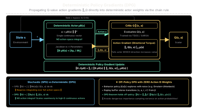
Deterministic policy gradients optimize continuous actions by propagating value gradients directly into actor weights via the chain rule, avoiding action integration.

Why Does This Exist?

In classical policy gradient methods (such as REINFORCE or standard Actor-Critic), policies are modeled as stochastic distributions $\pi_\theta(a \mid s)$ , mapping states to probability densities over actions.

According to the classical Policy Gradient Theorem (Sutton et al., 1999), the policy gradient integrates over both the state space and the entire action space:

$\nabla_\theta J(\pi_\theta) = \int_{\mathcal{S}} \rho^\pi(s) \int_{\mathcal{A}} \nabla_\theta \pi_\theta(a \mid s) Q^\pi(s, a) \, da \, ds$

In high-dimensional continuous action spaces—such as a 30-joint humanoid robot or continuous flight control—this formulation encounters severe bottlenecks:

Curse of Action Dimensionality: Estimating expectations over continuous action volumes requires vast sample counts, leading to immense gradient variance.
Intractable Off-Policy Importance Sampling: Reusing historical data off-policy requires weighting transitions by the likelihood ratio $\frac{\pi_\theta(a \mid s)}{\beta(a \mid s)}$ . Over continuous multi-dimensional spaces, these ratios fluctuate wildly or explode to infinity, destabilizing training.

David Silver et al. (2014) introduced the Deterministic Policy Gradient (DPG) framework to solve this. Instead of sampling actions from a probability density, the actor is formulated as a deterministic mapping:

$\mu_\theta: \mathcal{S} \to \mathcal{A}$

Because the policy outputs a single deterministic action vector rather than a distribution, the policy gradient integrates only over the state space. By applying the multivariate chain rule, the critic's gradient with respect to action $\nabla_a Q(s, a)$ acts as directional torque, backpropagating directly into the actor's weights.

Crucially, off-policy DPG requires zero importance sampling on action probabilities, making deterministic actor-critic algorithms (such as DDPG and TD3) remarkably sample-efficient in continuous control.

Think of It Like This

Steering Wheel Angle vs. Spinning a Roulette Wheel

Imagine learning to steer a high-performance race car around a fast, sharp corner.

If you operated under a Stochastic Policy Gradient (the roulette wheel): You would drive by spinning a roulette wheel centered around your current steering angle ( $a \sim \mathcal{N}(\mu, \sigma^2)$ ). At every millisecond, you randomly twitch the wheel slightly left or right. If a random twitch happened to round the bend safely without spinning out, the algorithm nudges the probability distribution toward that twitch. In a chassis with 30 independent steering joints, you would be spinning 30 simultaneous roulette wheels, requiring millions of trial-and-error crashes to discern which specific joint angle helped or hurt.

With Deterministic Policy Gradients (direct tactile torque): You grip a physical steering wheel rigidly connected to the front tires. As you enter the corner, you feel immediate tactile power-steering resistance through the steering column ( $\nabla_a Q(s, a)$ ). That physical torque tells you instantly: "Turning 5 degrees left will maximize tire friction and speed; turning right will lose traction."

You do not need to sample 50 random steering angles to find out—the road grip gradient directly instructs your arm muscles ( $\nabla_\theta \mu$ ) which way to turn the wheel.

Where the analogy stops: Tactile feedback in physical driving originates from mechanical tire friction. In DPG, $\nabla_a Q(s, a)$ is the analytical derivative of a learned neural network Critic evaluated at the actor's current continuous output $a = \mu_\theta(s)$ .

How It Actually Works

The Mathematical Mechanism: The DPG Theorem

Let $\mu_\theta: \mathcal{S} \to \mathcal{A}$ be a deterministic policy parameterized by $\theta \in \mathbb{R}^d$ . The continuous performance objective is the expected return under stationary state distribution $\rho^\mu(s)$ :

$J(\mu_\theta) \doteq \int_{\mathcal{S}} \rho^\mu(s) r(s, \mu_\theta(s)) \, ds$

The Deterministic Policy Gradient Theorem (Silver et al., 2014) proves that the gradient of this objective with respect to parameters $\theta$ is:

$\nabla_\theta J(\mu_\theta) = \int_{\mathcal{S}} \rho^\mu(s) \nabla_\theta \mu_\theta(s) \left. \nabla_a Q^\mu(s, a) \right|_{a = \mu_\theta(s)} \, ds$

In expectation form over state visitations:

$\nabla_\theta J(\mu_\theta) = \mathbb{E}_{s \sim \rho^\mu} \left[ \nabla_\theta \mu_\theta(s) \left. \nabla_a Q^\mu(s, a) \right|_{a = \mu_\theta(s)} \right]$

Where:

$\nabla_\theta \mu_\theta(s) \in \mathbb{R}^{d \times |\mathcal{A}|}$ is the Jacobian matrix of the deterministic actor network.
$\left. \nabla_a Q^\mu(s, a) \right|_{a = \mu_\theta(s)} \in \mathbb{R}^{|\mathcal{A}|}$ is the gradient of the action-value function with respect to action vector $a$ , evaluated at the actor's current choice $a = \mu_\theta(s)$ .
By the multivariate chain rule, $\nabla_a Q$ points in the direction of action space that increases value, and $\nabla_\theta \mu$ rotates that direction back into parameter space.

The Off-Policy DPG Formulation

To explore, an agent must collect experience using a stochastic exploratory behavior policy $\beta(a \mid s) \neq \mu_\theta(s)$ . The off-policy objective is:

$J_\beta(\mu_\theta) \doteq \int_{\mathcal{S}} \rho^\beta(s) Q^\mu(s, \mu_\theta(s)) \, ds$

Differentiating yields the Off-Policy Deterministic Policy Gradient:

$\nabla_\theta J_\beta(\mu_\theta) \approx \mathbb{E}_{s \sim \rho^\beta} \left[ \nabla_\theta \mu_\theta(s) \left. \nabla_a Q^\mu(s, a) \right|_{a = \mu_\theta(s)} \right]$

Because the target policy $\mu_\theta$ is deterministic, actions are evaluated directly through function composition $Q(s, \mu_\theta(s))$ . Consequently, no importance sampling ratio over actions ( $\frac{\pi(a \mid s)}{\beta(a \mid s)}$ ) is needed! Replay buffer samples from arbitrary historical behavior policies train the deterministic actor without variance explosion.

Worked Numerical Example

Consider a 1D continuous action environment ( $s \in \mathbb{R}, a \in \mathbb{R}$ ):

Current State: $s = 2.0$ .
Deterministic Actor: $\mu_\theta(s) = \theta_1 \cdot s + \theta_2$ .
Actor Parameters: $\theta_1 = 1.0, \theta_2 = 0.5$ .
Optimal Target Action: $s^* = 5.0$ .
Critic Function: $Q(s, a) = - (a - s^*)^2$ .
Learning Rate: $\alpha = 0.1$ .

Step 1: Forward Action Generation

The actor outputs continuous action: $a = \mu_\theta(s) = 1.0(2.0) + 0.5 = 2.50$

Current value evaluation: $Q(s, a) = - (2.50 - 5.0)^2 = - (-2.50)^2 = -6.2500$

Step 2: Critic Action Gradient (Directional Torque)

Differentiate the critic with respect to action $a$ : $\nabla_a Q(s, a) = \frac{\partial}{\partial a} \left[ -(a - 5.0)^2 \right] = -2(a - 5.0)$

Evaluated at $a = 2.50$ : $\left. \nabla_a Q(s, a) \right|_{a = 2.50} = -2(2.50 - 5.0) = -2(-2.50) = +5.00$

The critic informs the actor: "Increasing action $a$ by $+1.0$ will increase the Q-value with slope $+5.00$ ."

Step 3: Actor Parameter Jacobians

Differentiate the actor output with respect to its weights: $\nabla_{\theta_1} \mu(s) = \frac{\partial}{\partial \theta_1} [\theta_1 s + \theta_2] = s = 2.00$ $\nabla_{\theta_2} \mu(s) = \frac{\partial}{\partial \theta_2} [\theta_1 s + \theta_2] = 1.00$

Step 4: Deterministic Policy Gradient via Chain Rule

Apply the DPG theorem: $\nabla_{\theta_1} J = \nabla_{\theta_1} \mu(s) \cdot \nabla_a Q(s, a) = 2.00 \times 5.00 = 10.0000$ $\nabla_{\theta_2} J = \nabla_{\theta_2} \mu(s) \cdot \nabla_a Q(s, a) = 1.00 \times 5.00 = 5.0000$

Step 5: Gradient Ascent Parameter Update ( $\alpha = 0.1$ )

$\theta_1 \leftarrow \theta_1 + \alpha \nabla_{\theta_1} J = 1.00 + 0.1 \times 10.00 = 2.00$ $\theta_2 \leftarrow \theta_2 + \alpha \nabla_{\theta_2} J = 0.50 + 0.1 \times 5.00 = 1.00$

Step 6: Post-Update Evaluation

Evaluate the updated actor on state $s = 2.0$ : $a_{\text{new}} = \mu_{\theta_{\text{new}}}(2.0) = 2.00(2.0) + 1.00 = 5.00$

New Q-value: $Q(s, a_{\text{new}}) = -(5.00 - 5.00)^2 = 0.0000$

In a single gradient ascent step, the deterministic actor propagated the critic's action gradient through its parameters to converge directly to the optimal continuous action ( $a^* = 5.0$ ).

Code

1from typing import Tuple2
3
4class DeterministicActorCritic:5    """1D continuous action actor-critic verifying the Deterministic Policy Gradient theorem."""6
7    def __init__(self, theta1: float = 1.0, theta2: float = 0.5, s_star: float = 5.0) -> None:8        self.theta1 = theta19        self.theta2 = theta210        self.s_star = s_star11
12    def actor(self, s: float) -> float:13        """Deterministic policy: mu_theta(s) = theta1 * s + theta2."""14        return self.theta1 * s + self.theta215
16    def critic(self, s: float, a: float) -> float:17        """Critic value evaluator: Q(s, a) = - (a - s_star)^2."""18        return -((a - self.s_star) ** 2)19
20    def critic_action_grad(self, s: float, a: float) -> float:21        """Analytical gradient of Q w.r.t action: nabla_a Q(s, a) = - 2 * (a - s_star)."""22        return -2.0 * (a - self.s_star)23
24    def actor_param_grads(self, s: float) -> Tuple[float, float]:25        """Jacobian of actor output w.r.t parameters: [nabla_theta1 mu, nabla_theta2 mu]."""26        return s, 1.027
28    def policy_gradient(self, s: float) -> Tuple[float, float]:29        """DPG chain rule: nabla_theta J = nabla_theta mu(s) * nabla_a Q(s, a)|_{a = mu(s)}."""30        a = self.actor(s)31        grad_a_q = self.critic_action_grad(s, a)32        grad_t1_mu, grad_t2_mu = self.actor_param_grads(s)33
34        grad_theta1 = grad_t1_mu * grad_a_q35        grad_theta2 = grad_t2_mu * grad_a_q36        return grad_theta1, grad_theta237
38    def finite_difference_gradient(self, s: float, eps: float = 1e-6) -> Tuple[float, float]:39        """Numerical verification of J(theta) w.r.t parameters via finite differences."""40        base_a = self.actor(s)41        base_q = self.critic(s, base_a)42
43        # Perturb theta144        self.theta1 += eps45        q_t1 = self.critic(s, self.actor(s))46        fd_t1 = (q_t1 - base_q) / eps47        self.theta1 -= eps48
49        # Perturb theta250        self.theta2 += eps51        q_t2 = self.critic(s, self.actor(s))52        fd_t2 = (q_t2 - base_q) / eps53        self.theta2 -= eps54
55        return fd_t1, fd_t256
57    def update(self, s: float, alpha: float = 0.1) -> Tuple[float, float]:58        """Perform 1 gradient ascent step on actor parameters."""59        grad_t1, grad_t2 = self.policy_gradient(s)60        self.theta1 += alpha * grad_t161        self.theta2 += alpha * grad_t262        return self.theta1, self.theta263
64
65if __name__ == "__main__":66    s = 2.067    ac = DeterministicActorCritic(theta1=1.0, theta2=0.5, s_star=5.0)68
69    # Initial state evaluation70    a_init = ac.actor(s)71    q_init = ac.critic(s, a_init)72    print(f"Initial: theta1={ac.theta1:.2f}, theta2={ac.theta2:.2f} -> action a={a_init:.2f}, Q={q_init:.4f}")73
74    # Action gradient from Critic75    grad_a = ac.critic_action_grad(s, a_init)76    print(f"Critic action gradient nabla_a Q: {grad_a:.2f}")77
78    # Compare analytical DPG against finite-difference numerical gradients79    grad_t1, grad_t2 = ac.policy_gradient(s)80    fd_t1, fd_t2 = ac.finite_difference_gradient(s)81    print(f"Analytical DPG gradients: [grad_theta1={grad_t1:.4f}, grad_theta2={grad_t2:.4f}]")82    print(f"Finite Diff gradients:   [fd_theta1={fd_t1:.4f}, fd_theta2={fd_t2:.4f}]")83
84    # Gradient ascent update (alpha = 0.1)85    ac.update(s, alpha=0.1)86    a_new = ac.actor(s)87    q_new = ac.critic(s, a_new)88    print(f"After update (alpha=0.1): theta1={ac.theta1:.2f}, theta2={ac.theta2:.2f} -> action a={a_new:.2f}, Q={q_new:.4f}")

1# Expected Output:2# Initial: theta1=1.00, theta2=0.50 -> action a=2.50, Q=-6.25003# Critic action gradient nabla_a Q: 5.004# Analytical DPG gradients: [grad_theta1=10.0000, grad_theta2=5.0000]5# Finite Diff gradients:   [fd_theta1=10.0000, fd_theta2=5.0000]6# After update (alpha=0.1): theta1=2.00, theta2=1.00 -> action a=5.00, Q=-0.0000

Watch Out For

The Deterministic Exploration Paradox

By definition, a deterministic policy $\mu_\theta(s)$ outputs the exact same action every time it encounters state $s$ . If trained strictly on-policy, a deterministic actor cannot explore alternative continuous actions, causing learning to freeze prematurely in the nearest local optimum.

Furthermore, naive on-policy data collection cannot estimate $\nabla_a Q(s, a)$ away from the current path.

The Fix: DPG must be trained off-policy. The agent decouples exploration from learning by collecting transitions using an exploratory behavior policy:

$\beta(a \mid s) \doteq \mu_\theta(s) + \mathcal{N}_t$

Where $\mathcal{N}_t$ is an exploratory noise process (such as temporally correlated Ornstein-Uhlenbeck noise in DDPG, or uncorrelated Gaussian noise $\mathcal{N}(0, \sigma^2)$ in TD3).

Transitions $(s, a, r, s')$ are stored in an experience replay buffer. The critic trains on the noisy actions stored in replay, while the actor is updated off-policy via DPG by querying the critic's gradient $\nabla_a Q(s, \mu_\theta(s))$ on mini-batch states without requiring action importance sampling weights.

The Quick Version

Zero Action Integration: Unlike stochastic policy gradients that integrate over continuous action spaces, DPG integrates only over states ( $\nabla_\theta J = \mathbb{E}[\nabla_\theta \mu(s) \nabla_a Q(s, a)]$ ).
Direct Gradient Backpropagation: The critic's action gradient $\nabla_a Q(s, a)$ tells the actor which direction increases value; the multivariate chain rule propagates this signal directly into actor weights.
Off-Policy Sample Efficiency: Because the target policy is deterministic, off-policy replay buffer training does not require high-variance importance sampling ratios on continuous actions.
Requires Exploratory Behavior: Deterministic policies cannot explore on-policy; agents must inject external noise (Gaussian or Ornstein-Uhlenbeck) during data collection to ensure state-action coverage.