Implicit Q-Learning (IQL)
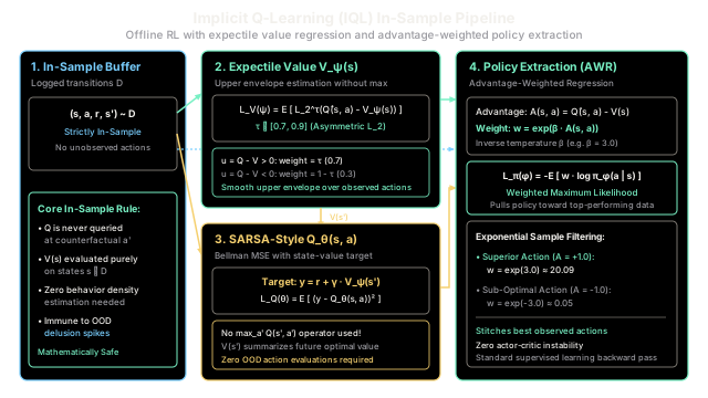
Instead of guessing what might happen for unobserved actions, Implicit Q-Learning fits an upper envelope over observed actions and extracts policy improvements completely in-sample.
Why Does This Exist?
In offline reinforcement learning, the central challenge is avoiding out-of-distribution (OOD) actions. Prior methods developed complex defenses to protect the value function against OOD hallucinations:
- Policy constraint methods (BCQ, BEAR) fit explicit density estimators (such as conditional Variational Autoencoders) to approximate the behavior distribution , rejecting candidate actions outside that distribution. However, generative modeling in high dimensions introduces severe density approximation errors and slows down training.
- Conservative value methods (CQL) add an explicit optimization penalty that depresses -values for unvisited actions. While theoretically sound, CQL requires sampling actions from uniform or adversarial distributions, making hyperparameter tuning difficult across heterogeneous environments.
Both approaches share a common vulnerability: they attempt to handle unobserved actions by explicitly modeling or penalizing them.
Implicit Q-Learning (IQL) (Kostrikov, Nair, & Levine, 2021) completely eliminates this vulnerability through a simple theoretical insight: an offline RL algorithm never needs to evaluate an unobserved action.
By decoupling state-value learning from action-maximization via asymmetric expectile regression, IQL estimates the upper envelope of values strictly across observed transitions. The entire training pipeline—value learning, Q-learning, and policy extraction—operates 100% in-sample, bypassing OOD actions altogether.
Think of It Like This
Finding the fastest city route from existing GPS trip logs
Imagine you are building a navigation system to find the fastest route across a city, but you only have access to a static log of 10,000 GPS trips driven by local cab drivers. You cannot send test cars onto the road during training.
-
Standard Off-Policy RL: Draws straight lines between GPS waypoints right through rivers, parks, and building walls. Because the algorithm has never seen a car try to drive through a brick wall, its random neural network extrapolations predict an impossibly fast 30-second commute. The planner chooses this hallucinatory route and crashes when deployed.
-
Conservative RL: Erects digital concrete barriers around every street not present in the dataset, which keeps the car safe but can over-penalize valid turns if data coverage is sparse.
-
The IQL Approach (In-Sample Expectile Filtering): The algorithm never considers driving off-road. Instead, it looks strictly at the roads drivers actually traveled. For any given intersection, instead of taking the average travel time, it computes the 80th percentile fastest trips (the upper expectile ) among the recorded drives.
Then, it trains the routing policy by imitating only those trips that matched or exceeded the 80th percentile travel times (Advantage-Weighted Regression), ignoring sluggish rides. The resulting navigation policy reproduces only the best observed driving maneuvers without ever inventing fictitious shortcuts.
Where the analogy stops: City streets have crisp geographical boundaries (paved asphalt vs. rivers). In continuous high-dimensional control tasks (such as robotic arm manipulation), there are no rigid physical road borders. Neural networks must use continuous expectile loss functions to smoothly approximate upper envelopes across continuous action manifolds.
How It Actually Works
The In-Sample Expectile Formulation and Three-Step Pipeline
IQL structures offline reinforcement learning into three modular, in-sample optimization steps that execute concurrently:
┌─────────────────────────────────────────────────────────────────┐│ 1. EXPECTILE VALUE REGRESSION (State Value V_ψ) ││ L_V(ψ) = E_{(s, a)~D} [ L_2^τ( Q_θ̂(s, a) - V_ψ(s) ) ] ││ Fits upper expectile (τ ∈ [0.7, 0.9]) purely on data actions │└──────────────────────────────┬──────────────────────────────────┘ │ State value V_ψ(s') ▼┌─────────────────────────────────────────────────────────────────┐│ 2. SARSA-STYLE Q-LEARNING (Action-Value Q_θ) ││ L_Q(θ) = E_{(s, a, r, s')~D} [ (r + γ·V_ψ(s') - Q_θ(s, a))² ] ││ Target y = r + γ·V(s') queries V, NOT max_a' Q(s', a')! │└──────────────────────────────┬──────────────────────────────────┘ │ Advantage A(s, a) = Q_θ̂ - V_ψ ▼┌─────────────────────────────────────────────────────────────────┐│ 3. ADVANTAGE-WEIGHTED POLICY EXTRACTION (Actor π_φ) ││ L_π(φ) = -E_{(s, a)~D} [ exp(β·A(s, a)) · log π_φ(a | s) ] ││ Weighted supervised maximum likelihood (Supervised Learning) │└─────────────────────────────────────────────────────────────────┘Step 1: Expectile Value Regression
In standard dynamic programming, the state value function represents the maximum over all possible actions: . In offline settings, taking an explicit maximum evaluates unseen actions outside the data support.
IQL replaces the hard with an asymmetric expectile regression objective:
where is a target Q-network and the asymmetric squared loss is defined as:
- For , , which recovers standard mean squared error (estimating the conditional mean ).
- For (typically or ), errors where receive weight , while errors where receive a smaller weight .
- As , approaches —the upper envelope of action-values observed in the dataset—without ever querying a single action outside .
Step 2: In-Sample Q-Function Learning
Using the learned state value , the action-value function is trained via standard mean squared error using SARSA-style Bellman targets:
Because the target directly evaluates the state-value function on the observed successor state , no action is sampled at state . The algorithm is completely immune to the out-of-distribution maximization trap.
Step 3: Policy Extraction via Advantage-Weighted Regression (AWR)
Once and are trained, IQL extracts a policy that favors actions with high advantage:
The actor is trained by maximizing the advantage-weighted log-likelihood over the dataset:
where is an inverse temperature parameter.
- Actions that outperformed the state-value baseline () receive exponentially large weights .
- Sub-optimal actions () receive exponentially decayed weights .
- Policy extraction reduces to simple weighted supervised regression. It avoids actor-critic policy gradient instabilities and requires zero backpropagation through the Q-network.
Worked numerical example
Let us trace a single training iteration evaluating expectile loss, in-sample Q targets, and advantage weights.
Setup:
- Current state with two recorded transitions in dataset :
- Action : Target Q-value .
- Action : Target Q-value .
- Current value network prediction: .
- Hyperparameters: expectile parameter , inverse temperature , discount factor .
Step 1: Compute Asymmetric Expectile Loss on Dataset Actions
-
For Superior Action :
- Difference: .
- Since , the asymmetric indicator assigns weight :
-
For Sub-Optimal Action :
- Difference: .
- Since , the asymmetric indicator assigns weight :
Notice that the positive error penalty () is larger than the negative error penalty (), pulling the value baseline upward toward the superior action .
Step 2: Compute In-Sample Q Target
Consider a transition , where the value network evaluates the next state at :
No candidate action was queried for next state .
Step 3: Compute Advantage Weights for Policy Extraction
-
For Superior Action :
- Advantage: .
- Exponential policy weight:
-
For Sub-Optimal Action :
- Advantage: .
- Exponential policy weight:
Action receives a gradient weight larger than action during policy extraction (). The actor effectively filters out the sub-optimal behavior without needing to discard data.
Code
import mathfrom typing import Dict, Tuple
class ImplicitQLearningEngine: """Demonstrates the core mechanics of Implicit Q-Learning (IQL):
1. Asymmetric expectile value regression (in-sample envelope fitting) 2. SARSA-style Q-learning with state-value Bellman targets 3. Advantage-weighted policy extraction (AWR) """
def __init__( self, tau: float = 0.7, beta: float = 3.0, gamma: float = 0.9 ) -> None: self.tau = tau self.beta = beta self.gamma = gamma
def asymmetric_expectile_loss(self, diff: float) -> float: """Calculates asymmetric L_2^tau loss:
L_2^tau(u) = |tau - I(u < 0)| * u^2 """ weight = self.tau if diff >= 0.0 else (1.0 - self.tau) return weight * (diff**2)
def compute_in_sample_q_target(self, reward: float, next_v: float) -> float: """Calculates SARSA-style Q target using next-state value:
y_Q = r + gamma * V(s') """ return reward + self.gamma * next_v
def compute_policy_weight( self, q_val: float, v_val: float, clip_max: float = 100.0, ) -> Tuple[float, float]: """Calculates advantage A(s, a) = Q - V and exponential weight:
w = min(exp(beta * A), clip_max) """ advantage = q_val - v_val raw_weight = math.exp(self.beta * advantage) clipped_weight = min(raw_weight, clip_max) return advantage, clipped_weight
# Execute test scenario matching the worked numerical exampleengine = ImplicitQLearningEngine(tau=0.7, beta=3.0, gamma=0.9)
# State evaluation baselinev_current = 5.0q_superior = 6.0q_suboptimal = 4.0
# 1. Expectile Loss on Dataset Actionsdiff_sup = q_superior - v_current # +1.0diff_sub = q_suboptimal - v_current # -1.0
loss_sup = engine.asymmetric_expectile_loss(diff_sup)loss_sub = engine.asymmetric_expectile_loss(diff_sub)
print(f"Difference (u_sup): {diff_sup:+.1f} -> Expectile Loss: {loss_sup:.4f}")# -> Difference (u_sup): +1.0 -> Expectile Loss: 0.7000
print(f"Difference (u_sub): {diff_sub:+.1f} -> Expectile Loss: {loss_sub:.4f}")# -> Difference (u_sub): -1.0 -> Expectile Loss: 0.3000
# 2. In-Sample Q-Targetreward = 1.0next_state_v = 4.5q_target = engine.compute_in_sample_q_target(reward, next_state_v)print(f"In-Sample Q Target (r + gamma * V(s')): {q_target:.2f}")# -> In-Sample Q Target (r + gamma * V(s')): 5.05
# 3. Advantage-Weighted Policy Extractionadv_sup, weight_sup = engine.compute_policy_weight(q_superior, v_current)adv_sub, weight_sub = engine.compute_policy_weight(q_suboptimal, v_current)
print( f"Superior Action: Advantage = {adv_sup:+.1f}, Weight = {weight_sup:.4f}")# -> Superior Action: Advantage = +1.0, Weight = 20.0855
print( f"Sub-Optimal Action: Advantage = {adv_sub:+.1f}, Weight = {weight_sub:.4f}")# -> Sub-Optimal Action: Advantage = -1.0, Weight = 0.0498
# Verification assertionsassert round(loss_sup, 2) == 0.70assert round(loss_sub, 2) == 0.30assert round(q_target, 2) == 5.05assert round(adv_sup, 1) == 1.0assert round(adv_sub, 1) == -1.0assert round(weight_sup, 4) == 20.0855assert round(weight_sub, 4) == 0.0498Watch Out For
Hyperparameter Sensitivity: Balancing Expectile tau and Temperature beta
While IQL is remarkably stable compared to adversarial or generative offline RL methods, performance is sensitive to two hyperparameters: the expectile coefficient and the inverse temperature .
-
Extreme Expectile Setting (): Setting attempts to force to match the true maximum of the empirical data. On finite or noisy datasets, this overfits to single outlier actions with abnormally high recorded rewards, reintroducing high target variance. Conversely, setting pulls toward the dataset mean, turning policy extraction into plain behavioral cloning.
-
Unconstrained Temperature (): Setting too high causes numerical overflow in and forces the policy to collapse onto a single dataset transition per state, destroying generalization.
The Fix:
- For standard continuous control (D4RL benchmark), set (or for high-quality demonstration datasets).
- Set and always clamp the exponential advantage weight with an upper ceiling (e.g. ) to guarantee gradient stability.
The Quick Version
- Implicit Q-Learning (IQL) solves offline reinforcement learning completely in-sample, eliminating out-of-distribution (OOD) action queries during training.
- State values are learned via asymmetric expectile regression (), fitting the upper envelope () of observed action-values without taking an explicit maximum.
- Q-functions are updated using SARSA-style targets , which query state values rather than unconstrained action heads.
- The policy is extracted using Advantage-Weighted Regression (AWR), applying exponential advantage weights in standard supervised maximum likelihood.