Advanced and PhD-Level Topics in RL

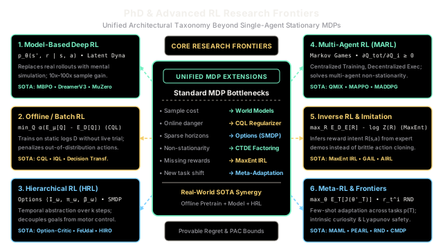
Why Does This Exist?

Foundational reinforcement learning conceptualizes intelligence through a single agent updating an unconstrained policy via trial-and-error inside a stationary, fully observed Markov Decision Process (MDP). While this classical paradigm powers milestone successes in video games and simplified physics benchmarks, it collapses when confronted with the realities of production engineering and physical autonomy.

Standard single-agent, model-free online algorithms suffer from five fundamental structural barriers:

1. Extreme Sample Inefficiency: Standard model-free policy gradients and Q-learning require tens of millions of environmental transitions. While trivial in video game emulators running at 5,000 frames per second, this sample appetite is fatal for physical robotics, where hardware wears out after thousands of cycles.
2. Online Trial-and-Error Hazard: In safety-critical sectors—such as surgical robotics, medical dosage planning, chemical refining, and autonomous driving—an untrained policy exploring random exploratory actions causes physical damage or loss of life.
3. Environment Non-Stationarity: When multiple agents operate in a shared arena (autonomous vehicle fleets, warehouse logistics, high-frequency market making), the actions of peer agents continuously alter the transition dynamics, invalidating the stationary transition assumption $P(s' \mid s, a)$.
4. Temporal Horizon and Credit Assignment Collapse: Flat policies that select motor actions at each millisecond fail over multi-hour horizons. When an agent receives an extrinsic reward only after 100,000 decisions, random exploratory noise has near-zero probability of reaching the objective.
5. Reward Specification Ambiguity: In complex human tasks, hand-crafting a scalar reward function $R(s, a)$ leads to severe reward hacking, where agents exploit loopholes in the objective rather than fulfilling human intent.

PhD-level and frontier reinforcement learning expands the mathematical formulation of the learning problem itself. By integrating latent world models, offline batch constraints, multi-agent game theory, temporal options, inverse reward inference, and meta-learning, these advanced architectures transition RL from toy academic simulators into scalable real-world intelligence.

Think of It Like This

How It Actually Works

The Six Research Frontiers of Modern RL

Modern advanced reinforcement learning decomposes beyond the standard MDP formulation into six complementary research pillars.

1                   ┌──────────────────────────────────────────────┐2                   │        The Advanced RL Research Frontier     │3                   └──────────────────────┬───────────────────────┘4          ┌───────────────────────────────┼───────────────────────────────┐5          │                               │                               │6┌─────────▼─────────┐           ┌─────────▼─────────┐           ┌─────────▼─────────┐7│ 1. World Models   │           │  2. Offline RL    │           │  3. Multi-Agent   │8│ Model-Based Latent│           │ Static Datasets D │           │ Markov Games &    │9│ Rollouts (Dreamer)│           │ CQL / IQL Bounds  │           │ CTDE (QMIX/MAPPO) │10└─────────┬─────────┘           └─────────┬─────────┘           └─────────┬─────────┘11          │                               │                               │12┌─────────▼─────────┐           ┌─────────▼─────────┐           ┌─────────▼─────────┐13│ 4. Hierarchical RL│           │  5. Inverse RL    │           │  6. Meta-RL & Safe│14│ Options & SMDPs   │           │ Infer Latent R(s) │           │ Task Generalize   │15│ (Option-Critic)   │           │ MaxEnt / GAIL     │           │ CMDPs & Curiosity │16└───────────────────┘           └───────────────────┘           └───────────────────┘

1. Model-Based Deep RL and Latent World Models

Model-free algorithms discard transitions immediately after computing Bellman TD errors. Model-based architectures explicitly learn the environmental transition dynamics $p_\theta(s_{t+1} \mid s_t, a_t)$ and reward function $r_\psi(s_t, a_t)$.

In Model-Based Policy Optimization (MBPO), an ensemble of bootstrap dynamics models $\{\hat{p}_{\theta_1}, \dots, \hat{p}_{\theta_M}\}$ is trained via maximum likelihood on a replay buffer of true physical interactions $\mathcal{D}_{\text{env}}$. The agent branches short $K$-step synthetic rollouts from sampled real states $s \in \mathcal{D}_{\text{env}}$ using the learned model, populating an imagined replay buffer $\mathcal{D}_{\text{model}}$.

The performance gap between the true policy return $\eta(\pi)$ and imagined return $\hat{\eta}(\pi)$ is bounded by the model generalization error $\epsilon_m = \max_{t} \mathbb{E}[D_{\text{TV}}(p \,\|\, \hat{p})]$ and policy divergence $\epsilon_\pi$:

In latent world models (e.g., DreamerV3), dynamics are modeled directly in a compact categorical or Gaussian latent representation $z_t \sim q_\phi(z_t \mid z_{t-1}, a_{t-1}, o_t)$ via Recurrent State Space Models (RSSM), enabling policy optimization entirely within imagined latent trajectories without rendering high-dimensional visual observations.

2. Offline / Batch Reinforcement Learning

Offline RL optimizes a policy from a fixed dataset $\mathcal{D} = \{(s, a, r, s')\}$ gathered by unknown historical behavior policies $\pi_\beta$, forbidding all online interaction during training.

The governing failure mode of standard off-policy RL in the batch setting is distributional shift. When computing Bellman backup targets:

the maximization operator queries actions $a'$ where data density $d^{\pi_\beta}(s', a') \approx 0$. Neural network value estimators extrapolate unpredictably in unconstrained out-of-distribution (OOD) action spaces, producing spurious overestimation spikes that compound recursively across Bellman updates.

Conservative Q-Learning (CQL) rectifies this by augmenting the temporal difference objective with an explicit value regularizer that penalizes expected Q-values under the current policy while maximizing Q-values on dataset state-action pairs:

where $\alpha > 0$ controls the trade-off. Kumar et al. proved that CQL yields provably conservative value lower bounds, $\hat{Q}^{\pi}(s, a) \le Q^\pi(s, a)$, guaranteeing that the learned policy never relies on ungrounded optimism.

3. Multi-Agent Reinforcement Learning (MARL)

Multi-agent environments are formalized as Markov Games (Stochastic Games) defined by a tuple $\langle \mathcal{N}, \mathcal{S}, \{\mathcal{A}_i\}_{i=1}^N, \mathcal{P}, \{R_i\}_{i=1}^N, \gamma \rangle$, where $N$ agents interact simultaneously.

Training independent learners fails because transition dynamics $P(s' \mid s, a_i, \mathbf{a}_{-i})$ non-stationarily fluctuate as peer agents update their respective policies $\pi_{-i}$. Modern MARL resolves this via Centralized Training with Decentralized Execution (CTDE):

• During Centralized Training: The critic observes the full joint state $\mathbf{s}$ and all joint actions $\mathbf{a} = (a_1, \dots, a_N)$.
• During Decentralized Execution: Individual actor networks select actions conditioned solely on private local observations: $a_i \sim \pi_i(a_i \mid o_i)$.

In cooperative cooperative multi-agent value factorization (e.g., QMIX), the joint action-value function $Q_{\text{tot}}(\mathbf{s}, \mathbf{a})$ is decomposed into individual agent utilities $Q_i(o_i, a_i)$ under the Individual-Global-Max (IGM) condition:

QMIX enforces IGM by restricting the factorization network weights to non-negative values via hypernetworks conditioned on the global state $\mathbf{s}$:

4. Hierarchical RL and Temporal Abstraction

Hierarchical RL decomposes monolithic policy search across multiple timescales using Semi-Markov Decision Processes (SMDPs).

Under the Options Framework, an option $\omega \in \Omega$ is defined by a triplet $\langle \mathcal{I}_\omega, \pi_\omega, \beta_\omega \rangle$:

• Initiation Set $\mathcal{I}_\omega \subseteq \mathcal{S}$: The environmental states in which the option can be launched.
• Internal Option Policy $\pi_\omega(a \mid s)$: Dictates primitive motor actions during the option's lifespan.
• Termination Condition $\beta_\omega: \mathcal{S} \to [0, 1]$: The probability that the option terminates upon reaching state $s$.

A high-level policy over options $\pi_\Omega(\omega \mid s)$ selects an option, which persists for a variable duration of $k$ timesteps. The SMDP Bellman optimality equation operates over this extended temporal horizon:

In goal-conditioned hierarchies (such as FeUdal Networks and HIRO), a Manager network generates latent goal vectors $g_t \in \mathbb{R}^d$ at interval $c$, while a low-level Worker receives intrinsic rewards for minimizing the directional distance between state transitions and the Manager's directional vector.

5. Inverse Reinforcement Learning (IRL) and Imitation

When task objectives are intricate or safety constraints cannot be reduced to hand-crafted mathematical formulas, engineers collect demonstrations from human or algorithmic experts: $\mathcal{D}_E = \{\tau_1, \dots, \tau_M\}$.

Directly predicting actions via supervised classification (Behavioral Cloning) suffers from compounding error $\mathcal{O}(T^2 \epsilon)$ over horizon $T$ due to covariate shift. Inverse Reinforcement Learning recovers the underlying latent reward function $R^*(s, a)$ that rationalizes the expert's behavior.

Under Maximum Entropy IRL, demonstrations are assumed to be sampled from a Boltzmann distribution over trajectory returns with maximum entropy to resolve reward ambiguity:

The learning objective maximizes the log-likelihood of expert trajectories:

Generative Adversarial Imitation Learning (GAIL) lifts this into a minimax game: a discriminator $D_\psi(s, a)$ learns to distinguish expert transitions from generated transitions, while a policy $\pi_\theta$ optimizes an RL objective using $-\log(1 - D_\psi(s, a))$ as an endogenous reward signal.

6. Meta-RL, Exploration Frontiers, and Safe Constraints

• Meta-RL (Learning to Learn): Rather than optimizing for a single MDP $\mathcal{M}$, the agent samples tasks from a distribution $p(\mathcal{T})$. Algorithms like MAML and PEARL optimize meta-parameters $\theta$ such that a single gradient update or latent context identification step $z \sim q_\phi(z \mid \tau_{1:t})$ adapts the policy to a novel MDP within a few transitions.
• Intrinsic Exploration: In zero-reward environments, agents generate self-supervised exploration bonuses. In Random Network Distillation (RND), a randomly initialized neural network $f(s)$ remains fixed while a predictor network $\hat{f}_\theta(s)$ is trained to predict $f(s)$. The prediction error serves as an intrinsic exploration reward: $$r_t^i = \left\| \hat{f}_\theta(s_{t+1}) - f(s_{t+1}) \right\|_2^2$$
• Safe Constrained MDPs (CMDPs): Optimization is framed as maximizing expected return subject to auxiliary cost budgets: $\mathbb{E}[R] \text{ subject to } \mathbb{E}[C_k] \le d_k$, solved via primal-dual Lagrangian formulations or Lyapunov barrier certificates.

Worked numerical example

To understand how these paradigms alter learning dynamics in practice, consider a benchmark grid domain with:

• State space size $|\mathcal{S}| = 200$
• Action space size $|\mathcal{A}| = 4$
• Discount factor $\gamma = 0.95$ (effective horizon $H \approx \frac{1}{1-\gamma} = 20$)
• Accuracy requirement $\epsilon = 0.50$ return units

Step 1: Theoretical Model-Free Sample Complexity

Under standard PAC-MDP (Probably Approximately Correct) sample complexity bounds for tabular and linear model-free Q-learning (Kakade, 2003):

Substituting our parameters:

• $(1 - \gamma) = 1.0 - 0.95 = 0.05$
• $(1 - \gamma)^3 = (0.05)^3 = 0.000125$
• $\epsilon^2 = (0.50)^2 = 0.25$
• Denominator product: $0.000125 \times 0.25 = 0.00003125$
• Numerator: $|\mathcal{S}| |\mathcal{A}| = 200 \times 4 = 800$

A model-free algorithm requires over $2.56 \times 10^7$ real physical environment interactions to guarantee near-optimal convergence.

Step 2: Model-Based Dyna Sample Efficiency Gain

Now suppose the agent fits an internal transition dynamics model $\hat{p}(s' \mid s, a)$ from collected real data. For every real physical interaction, the agent performs $K = 15$ synthetic rollout steps in latent imagination (Dyna / MBPO branching).

The effective training data volume generated is:

To supply the policy with the equivalent $25,600,000$ gradient-generating samples:

Physical wear on robotic actuators is reduced by $93.75\%$ through internal model rollouts.

Step 3: Offline RL Conservative Q-Learning (CQL) Penalty Calculation

Now suppose physical interaction is completely prohibited ($N_{\text{online}} = 0$). We train exclusively from a fixed historical dataset $\mathcal{D}$.

At a decision state $s_0$:

• The dataset contains historical records for in-distribution action $a_{\text{data}}$ with true Q-value: $$Q^*(s_0, a_{\text{data}}) = 10.00$$
• An unconstrained neural network extrapolates an out-of-distribution (OOD) action $a_{\text{ood}} \notin \mathcal{D}$ with an exaggerated, hallucinated value: $$\hat{Q}_{\text{raw}}(s_0, a_{\text{ood}}) = 18.50$$

In standard off-policy Q-learning, the policy greedily selects $\arg\max_a \hat{Q}(s_0, a) = a_{\text{ood}}$, resulting in an immediate policy failure upon real-world deployment.

CQL introduces an explicit value regularizer to the loss with weight $\alpha = 1.80$. Suppose the policy distribution $\mu$ assigns probability $\mu(a_{\text{ood}}) = 0.60$ and $\mu(a_{\text{data}}) = 0.40$:

1. Compute expected Q-value under the policy: $$\mathbb{E}_{a \sim \mu}[Q(s_0, a)] = 0.60 \times 18.50 + 0.40 \times 10.00 = 11.10 + 4.00 = 15.10$$
2. Compute expected Q-value under the dataset: $$\mathbb{E}_{a \sim \mathcal{D}}[Q(s_0, a)] = 1.00 \times 10.00 = 10.00$$
3. Compute the conservatism gap: $$\Delta_{\text{gap}} = \mathbb{E}_{\mu}[Q] - \mathbb{E}_{\mathcal{D}}[Q] = 15.10 - 10.00 = 5.10$$
4. Compute the regularizer loss penalty: $$\text{Loss Penalty} = \alpha \times \Delta_{\text{gap}} = 1.80 \times 5.10 = 9.18$$
5. Compute the penalized conservative Q-value for the OOD action: $$\hat{Q}_{\text{CQL}}(s_0, a_{\text{ood}}) = \hat{Q}_{\text{raw}}(s_0, a_{\text{ood}}) - \text{Loss Penalty} = 18.50 - 9.18 = 9.32$$

Comparing the final regularized action values:

• $\hat{Q}_{\text{CQL}}(s_0, a_{\text{data}}) = 10.00$
• $\hat{Q}_{\text{CQL}}(s_0, a_{\text{ood}}) = 9.32$

Because $10.00 > 9.32$, the policy greedily selects the verified dataset action $a_{\text{data}}$, suppressing the dangerous OOD extrapolation hallucination.

Code

The following pure Python script implements the comparative taxonomy evaluator, verifies sample complexity bounds and Dyna speedups, computes CQL regularizers, and enforces structural invariants across the six advanced paradigms.

1from dataclasses import dataclass2from typing import Dict, Tuple3
4@dataclass5class ParadigmProfile:6    name: str7    interaction_type: str8    sample_efficiency_rank: int9    solves_distribution_shift: bool10    supports_temporal_abstraction: bool11    multi_agent_capable: bool12
13class AdvancedRLTaxonomy:14    """Taxonomy evaluator comparing PhD-level Reinforcement Learning paradigms."""15
16    def __init__(self) -> None:17        self.paradigms: Dict[str, ParadigmProfile] = {18            "model_free_rl": ParadigmProfile(19                name="Model-Free Deep RL (PPO/SAC)",20                interaction_type="Online Trial-and-Error",21                sample_efficiency_rank=4,22                solves_distribution_shift=False,23                supports_temporal_abstraction=False,24                multi_agent_capable=False,25            ),26            "model_based_deep_rl": ParadigmProfile(27                name="Model-Based Deep RL (Dreamer/MBPO)",28                interaction_type="Online + Latent Imagination",29                sample_efficiency_rank=1,30                solves_distribution_shift=False,31                supports_temporal_abstraction=False,32                multi_agent_capable=False,33            ),34            "offline_rl": ParadigmProfile(35                name="Offline / Batch RL (CQL/IQL)",36                interaction_type="Zero Online Interaction (Fixed Log)",37                sample_efficiency_rank=2,38                solves_distribution_shift=True,39                supports_temporal_abstraction=False,40                multi_agent_capable=False,41            ),42            "hierarchical_rl": ParadigmProfile(43                name="Hierarchical RL (Options / FeUdal)",44                interaction_type="Online Semi-Markov Process",45                sample_efficiency_rank=3,46                solves_distribution_shift=False,47                supports_temporal_abstraction=True,48                multi_agent_capable=False,49            ),50            "multi_agent_rl": ParadigmProfile(51                name="Multi-Agent RL (QMIX/MAPPO)",52                interaction_type="Markov Games (CTDE)",53                sample_efficiency_rank=3,54                solves_distribution_shift=False,55                supports_temporal_abstraction=False,56                multi_agent_capable=True,57            ),58        }59
60    def compute_sample_complexity_mf(61        self,62        n_states: int,63        n_actions: int,64        gamma: float,65        epsilon: float,66    ) -> int:67        """Theoretical PAC-MDP sample complexity bound for model-free RL."""68        horizon_factor = (1.0 - gamma) ** 369        accuracy_factor = epsilon ** 270        bound = (n_states * n_actions) / (horizon_factor * accuracy_factor)71        return int(round(bound))72
73    def evaluate_dyna_speedup(74        self,75        samples_mf: int,76        imagined_steps_k: int,77    ) -> Tuple[int, float]:78        """Calculates physical environment interactions needed given K imagined rollouts per step."""79        real_samples = int(round(samples_mf / (1.0 + imagined_steps_k)))80        speedup = float(samples_mf) / float(real_samples)81        return real_samples, speedup82
83    def compute_cql_penalty(84        self,85        q_ood: float,86        q_data: float,87        prob_ood: float,88        prob_data: float,89        alpha: float,90    ) -> Tuple[float, float, float]:91        """Computes Conservative Q-Learning penalty on out-of-distribution state-action pairs."""92        expected_q_policy = prob_ood * q_ood + prob_data * q_data93        expected_q_dataset = q_data94        conservatism_gap = expected_q_policy - expected_q_dataset95        loss_penalty = alpha * conservatism_gap96        # Corrected conservative value estimate for OOD action97        q_cql_ood = q_ood - loss_penalty98        return conservatism_gap, loss_penalty, q_cql_ood99
100taxonomy = AdvancedRLTaxonomy()101
102# 1. Sample Complexity Benchmark (|S|=200, |A|=4, gamma=0.95, epsilon=0.50)103n_mf = taxonomy.compute_sample_complexity_mf(104    n_states=200, n_actions=4, gamma=0.95, epsilon=0.50105)106print(f"Model-Free Sample Bound: {n_mf:,} steps")107# -> Model-Free Sample Bound: 25,600,000 steps108
109# 2. Model-Based Speedup via K=15 Imagination Horizon110n_mb, speedup = taxonomy.evaluate_dyna_speedup(samples_mf=n_mf, imagined_steps_k=15)111print(f"Model-Based Real Steps: {n_mb:,} steps (Speedup: {speedup:.1f}x)")112# -> Model-Based Real Steps: 1,600,000 steps (Speedup: 16.0x)113
114# 3. Offline RL Conservatism under OOD Extrapolation (alpha=1.80)115gap, penalty, q_penalized = taxonomy.compute_cql_penalty(116    q_ood=18.5, q_data=10.0, prob_ood=0.6, prob_data=0.4, alpha=1.8117)118print(f"CQL Gap: {gap:.2f} | Penalty: {penalty:.2f} | Penalized Q(s, a_ood): {q_penalized:.2f}")119# -> CQL Gap: 5.10 | Penalty: 9.18 | Penalized Q(s, a_ood): 9.32120
121# 4. Assert Taxonomy Invariants122assert taxonomy.paradigms["offline_rl"].solves_distribution_shift is True123assert taxonomy.paradigms["hierarchical_rl"].supports_temporal_abstraction is True124assert taxonomy.paradigms["multi_agent_rl"].multi_agent_capable is True125print("All PhD RL taxonomy invariants verified successfully.")126# -> All PhD RL taxonomy invariants verified successfully.

Watch Out For

The Quick Version

• Model-Based Deep RL & World Models replace physical trial-and-error with internal latent rollouts, slashing environmental sample complexity by orders of magnitude while bounding model drift error.
• Offline / Batch RL trains high-performing policies strictly from static historical logs $\mathcal{D}$, utilizing conservative regularizers (CQL, IQL) to neutralize catastrophic out-of-distribution value overestimation.
• Multi-Agent Systems (MARL) address environment non-stationarity via Centralized Training with Decentralized Execution (CTDE) and monotonic value factorization (QMIX: $\frac{\partial Q_{\text{tot}}}{\partial Q_i} \ge 0$).
• Hierarchical and Meta-RL master long horizons through temporal options ($\langle \mathcal{I}_\omega, \pi_\omega, \beta_\omega \rangle$) and enable rapid adaptation across task families through learned priors and self-supervised intrinsic curiosity.

What to Read Next

• Advanced RL Paradigms
• Model-Based Deep RL
• Offline Reinforcement Learning
• Deep Reinforcement Learning