Dyna Architecture

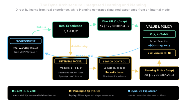
The Dyna architecture lets an agent learn twice from every experience: first directly through trial and error, and then dozens of times in the background by replaying what it learned inside an internal world model.

Why Does This Exist?

In real-world reinforcement learning, environment interactions are expensive, slow, and potentially hazardous. A physical robot attempting to learn solely through model-free trial and error (like standard Q-learning) requires hundreds of thousands of physical transitions to propagate rewards backwards across its state space.

Historically, reinforcement learning was divided into two isolated camps:

Model-Free RL (Direct Learning): The agent interacts with the real world, applies Bellman updates directly to value functions or policies, and discards the transition. It requires no world model, but its sample efficiency is notoriously poor.
Model-Based Planning (Dynamic Programming): The agent assumes a fully known transition model $P(s' \mid s, a)$ and reward model $R(s, a)$ , running offline sweeps across states. While sample efficient, it is helpless when the environment dynamics are initially unknown.

Introduced by Richard Sutton in 1990, the Dyna architecture bridges this divide by synthesizing direct learning, model learning, and planning into a single unified online architecture.

In Dyna, real experience serves a dual purpose:

It immediately updates the value function via direct model-free RL.
It simultaneously trains an internal world model $\text{Model}(s, a) \to (r, s')$ .

Between real environment steps, the agent pauses to run planning steps: it samples hypothetical state-action transitions from its learned model, generates simulated experiences, and applies the exact same reinforcement learning update rule to its value function. By "dreaming" $N$ simulated transitions for every single physical step, Dyna accelerates sample efficiency by orders of magnitude.

Think of It Like This

Flight Training: Daytime Cockpit Hours vs. Nighttime Flight Simulators

Imagine training to become a commercial airline pilot:

Pure Model-Free RL (Only Flying Real Planes): You learn solely by sitting in a physical cockpit. If you encounter severe crosswinds during a landing at 3:00 PM, you make a real-time adjustment. Once you park the plane, you wait until tomorrow's flight to experience crosswinds again. It takes years and hundreds of thousands of dollars in jet fuel to encounter enough rare weather conditions to become proficient.
Pure Model-Based Dynamic Programming (The Theoretical Textbook): You are handed a 2,000-page aerodynamic manual and expected to compute exact flight paths mathematically before ever touching a control stick. If the real atmosphere deviates from your equations, your plans fail.
The Dyna Architecture (Flying by Day, Simulating by Night): During the day, you fly real cockpit hours ( $S \to A \to R \to S'$ ). Each landing teaches your reflexes directly (Direct RL). Simultaneously, you plug your flight recorder's telemetry into a computer (Model Learning). That evening, you sit in a high-fidelity flight simulator that replicates the exact wind shear and turbulence you recorded that afternoon (Planning). In one evening, you rehearse that crosswind approach 50 times in simulation ( $N = 50$ ). By tomorrow morning, your reflexes are already sharpened without burning a single extra drop of fuel.

Where the analogy stops: A human flight simulator uses complex physics engines, whereas tabular Dyna-Q builds a lookup table of past $(s, a) \to (r, s')$ observations. Furthermore, Dyna applies identical temporal difference update equations to both real and simulated transitions.

How It Actually Works

Sutton's Dyna-Q Algorithm and Dyna-Q+ Exploration

The Dyna architecture operates on two concurrent timescales: real environment time and background planning time. In tabular Dyna-Q, the agent maintains an action-value table $Q(s, a)$ and a deterministic transition model $\text{Model}(s, a)$ .

1. The Core Dyna-Q Loop

At each discrete time step $t$ , the agent executes the following unified procedure:

Action Selection: Select an action $A$ in state $S$ using an exploratory policy (e.g., $\varepsilon$ -greedy with respect to $Q$ ): $A \leftarrow \pi(S)$
Real Interaction: Execute $A$ in the real environment; observe real scalar reward $R$ and next state $S'$ .
Direct RL Update: Apply a standard Q-learning update to the Q-table using the real transition: $Q(S, A) \leftarrow Q(S, A) + \alpha \left[ R + \gamma \max_{a'} Q(S', a') - Q(S, A) \right]$
Model Learning: Store the observed transition in the internal model buffer: $\text{Model}(S, A) \leftarrow (R, S')$ The agent also tracks that state $S$ and action $A$ have been experienced, adding them to sets $\mathcal{S}_{\text{visited}}$ and $\mathcal{A}_{\text{visited}}(S)$ .
Background Planning Loop (Repeat $N$ Times):
- Search Control: Sample a previously visited state $s$ uniformly at random from $\mathcal{S}_{\text{visited}}$ .
- Sample a previously executed action $a$ uniformly at random from $\mathcal{A}_{\text{visited}}(s)$ .
- Simulate: Query the internal model for the predicted outcome: $(r, s') \leftarrow \text{Model}(s, a)$
- Planning Update: Apply the standard Q-learning Bellman update to $Q(s, a)$ using simulated experience: $Q(s, a) \leftarrow Q(s, a) + \alpha \left[ r + \gamma \max_{a'} Q(s', a') - Q(s, a) \right]$
State Transition: Set $S \leftarrow S'$ and repeat.

When $N = 0$ , Dyna-Q reduces exactly to standard model-free Q-learning. When $N > 0$ , each physical transition is amplified by $N$ simulated replay updates.

2. Dyna-Q+: Exploration in Non-Stationary Worlds

A major challenge for model-based planning arises when the real world changes (non-stationary environments):

Shortcuts open: A wall vanishes, opening a faster path to the goal.
Paths block: An existing corridor is closed off.

A standard Dyna-Q agent whose model was trained on the old environment will continue planning with outdated transitions, failing to discover new shortcuts because its greedy policy avoids unvisited areas.

To overcome this, Sutton formulated Dyna-Q+, which introduces an exploration bonus based on recency. Let $\tau(s, a)$ be the number of real time steps that have elapsed since state-action pair $(s, a)$ was last executed in the real environment.

During planning, the model's simulated reward is augmented with a bonus proportional to the square root of elapsed time:

$r_{\text{bonus}} = r + \kappa \sqrt{\tau(s, a)}$

Where:

$\tau(s, a)$ measures elapsed time since $(s, a)$ was tried physically.
$\kappa > 0$ is a small exploration scaling coefficient (e.g., $10^{-4}$ ).

The longer a transition has gone unvisited, the more attractive it becomes during background planning. If a dormant action suddenly yields a high bonus in simulation, the agent's policy shifts toward visiting that action in the real world to test whether the environment has changed.

Worked numerical example

To observe how background planning propagates rewards across multiple states in a single real transition, consider a 3-state navigation corridor:

$S_0 \xrightarrow{\text{right}} S_1 \xrightarrow{\text{right}} S_2 \text{ (Terminal Goal, Reward } +10.0\text{)}$

Parameters:

Discount factor $\gamma = 0.9$
Learning rate $\alpha = 0.5$
Initial Q-values: $Q(s, a) = 0.0$ for all states
Action: $A = \text{"right"}$

Step 1: Real Step from $S_0$ to $S_1$ (Reward $R_1 = 0.0$ )

Direct RL: $Q(S_0, \text{right}) \leftarrow 0.0 + 0.5 \left[ 0.0 + 0.9 \max Q(S_1) - 0.0 \right] = 0.0000$
Model Storage: $\text{Model}(S_0, \text{right}) \leftarrow (0.0, S_1)$
Visited memory: $\mathcal{S}_{\text{visited}} = \{S_0\}$ . Planning updates on $(S_0, \text{right})$ yield TD error 0.

Step 2: Real Step from $S_1$ to $S_2$ (Terminal Goal, Reward $R_2 = 10.0$ )

Direct RL Update: $Q(S_1, \text{right}) \leftarrow 0.0 + 0.5 \left[ 10.0 + 0.9(0.0) - 0.0 \right] = \mathbf{5.0000}$
Model Storage: $\text{Model}(S_1, \text{right}) \leftarrow (10.0, S_2)$
Visited memory: $\mathcal{S}_{\text{visited}} = \{S_0, S_1\}$ .

Now compare what happens next with $N = 0$ (No Planning) versus $N = 5$ (Dyna Planning):

Case 1: Pure Q-Learning ( $N = 0$ )

No planning steps are executed.

Values at end of Episode 1: $Q(S_1, \text{right}) = 5.0000, \quad Q(S_0, \text{right}) = \mathbf{0.0000}$
State $S_0$ learned nothing from the agent reaching the goal. It will require a second physical episode just for $S_0$ to discover that $S_1$ has positive value.

Case 2: Dyna-Q Planning ( $N = 5$ Simulated Steps)

The agent pauses in the background to execute 5 simulated planning steps, sampling from $\mathcal{S}_{\text{visited}} = \{S_0, S_1\}$ :

Planning Step 1 (Sample $S_0$ ):
- Query model: $(r=0.0, s'=S_1)$ .
- Target: $r + \gamma \max Q(S_1) = 0.0 + 0.9(5.0000) = 4.5000$ .
- Update: $Q(S_0, \text{right}) \leftarrow 0.0 + 0.5(4.5000 - 0.0) = \mathbf{2.2500}$ . (The goal reward has already leaped backward to $S_0$ without any physical movement!)
Planning Step 2 (Sample $S_1$ ):
- Query model: $(r=10.0, s'=S_2)$ . Target: $10.0 + 0.0 = 10.0$ .
- Update: $Q(S_1, \text{right}) \leftarrow 5.0 + 0.5(10.0 - 5.0) = \mathbf{7.5000}$ .
Planning Step 3 (Sample $S_0$ ):
- Query model: $(r=0.0, s'=S_1)$ . Target: $0.9(7.5000) = 6.7500$ .
- Update: $Q(S_0, \text{right}) \leftarrow 2.2500 + 0.5(6.7500 - 2.2500) = \mathbf{4.5000}$ .
Planning Step 4 (Sample $S_1$ ):
- Target: $10.0$ .
- Update: $Q(S_1, \text{right}) \leftarrow 7.5000 + 0.5(10.0 - 7.5000) = \mathbf{8.7500}$ .
Planning Step 5 (Sample $S_0$ ):
- Target: $0.9(8.7500) = 7.8750$ .
- Update: $Q(S_0, \text{right}) \leftarrow 4.5000 + 0.5(7.8750 - 4.5000) = \mathbf{6.1875}$ .

Comparison at the End of Episode 1

Algorithm	$Q(S_0, \text{right})$	$Q(S_1, \text{right})$	Episodes Needed for $S_0$ to Learn
Q-Learning ( $N = 0$ )	$0.0000$	$5.0000$	2 episodes
Dyna-Q ( $N = 5$ )	$\mathbf{6.1875}$	$\mathbf{8.7500}$	1 episode

With 5 background planning steps, $S_0$ absorbed over $60\%$ of the optimal return during the very first physical run.

Code

The following self-contained Python implementation trains a Dyna-Q agent on a discrete gridworld, contrasting $N=0$ against $N=5$ planning steps and asserting sample efficiency gains.

1import random2from typing import Dict, List, Set, Tuple3
4
5class DynaQAgent:6    """Tabular Dyna-Q agent integrating direct RL with background model planning.7
8    Environment: 0 <-> 1 <-> 2 <-> 3 (Terminal Goal, Reward = +10.0)9    Actions: 0 = 'left', 1 = 'right'10    """11
12    def __init__(13        self,14        num_states: int = 4,15        planning_steps: int = 5,16        alpha: float = 0.5,17        gamma: float = 0.9,18        epsilon: float = 0.0,19    ) -> None:20        self.num_states = num_states21        self.goal_state = num_states - 122        self.actions = [0, 1]  # 0: left, 1: right23        self.planning_steps = planning_steps24        self.alpha = alpha25        self.gamma = gamma26        self.epsilon = epsilon27
28        # Action-value table Q(s, a)29        self.q_table: Dict[Tuple[int, int], float] = {30            (s, a): 0.0 for s in range(num_states) for a in self.actions31        }32
33        # Deterministic transition model: (s, a) -> (reward, next_state)34        self.model: Dict[Tuple[int, int], Tuple[float, int]] = {}35
36        # History tracking for search control sampling37        self.observed_states: Set[int] = set()38        self.observed_actions: Dict[int, Set[int]] = {}39
40    def choose_action(self, state: int) -> int:41        """Epsilon-greedy policy that breaks ties toward 'right' (1)."""42        if random.random() < self.epsilon:43            return random.choice(self.actions)44        q_left = self.q_table[(state, 0)]45        q_right = self.q_table[(state, 1)]46        return 1 if q_right >= q_left else 047
48    def step_environment(49        self, state: int, action: int50    ) -> Tuple[int, float, bool]:51        """Real environment step dynamics."""52        next_state = (53            min(state + 1, self.goal_state)54            if action == 155            else max(state - 1, 0)56        )57        done = next_state == self.goal_state58        reward = 10.0 if done else 0.059        return next_state, reward, done60
61    def direct_rl_update(62        self, s: int, a: int, r: float, s_next: int, done: bool63    ) -> None:64        """Applies direct Q-learning Bellman update from real experience."""65        max_q_next = (66            0.067            if done68            else max(self.q_table[(s_next, act)] for act in self.actions)69        )70        td_error = r + self.gamma * max_q_next - self.q_table[(s, a)]71        self.q_table[(s, a)] += self.alpha * td_error72
73    def update_model(self, s: int, a: int, r: float, s_next: int) -> None:74        """Stores transition in model and records visited history."""75        self.model[(s, a)] = (r, s_next)76        self.observed_states.add(s)77        if s not in self.observed_actions:78            self.observed_actions[s] = set()79        self.observed_actions[s].add(a)80
81    def planning_loop(self) -> None:82        """Simulates N hypothetical transitions from learned model."""83        for _ in range(self.planning_steps):84            # Search Control: sample previously visited state and action85            sim_s = random.choice(list(self.observed_states))86            sim_a = random.choice(list(self.observed_actions[sim_s]))87
88            # Query internal model89            sim_r, sim_s_next = self.model[(sim_s, sim_a)]90            sim_done = sim_s_next == self.goal_state91
92            # Apply identical Q-learning update using simulated experience93            max_q_next = (94                0.095                if sim_done96                else max(self.q_table[(sim_s_next, act)] for act in self.actions)97            )98            td_error = sim_r + self.gamma * max_q_next - self.q_table[(sim_s, sim_a)]99            self.q_table[(sim_s, sim_a)] += self.alpha * td_error100
101    def run_episode(self) -> int:102        """Executes one episode of real interaction, model learning, and planning."""103        state = 0104        step_count = 0105        while state != self.goal_state and step_count < 50:106            action = self.choose_action(state)107            next_state, reward, done = self.step_environment(state, action)108
109            # 1. Direct RL110            self.direct_rl_update(state, action, reward, next_state, done)111
112            # 2. Model learning113            self.update_model(state, action, reward, next_state)114
115            # 3. Background planning (N simulated updates)116            self.planning_loop()117
118            state = next_state119            step_count += 1120
121        return step_count122
123
124# Compare Q-learning (N=0) against Dyna-Q (N=5) in Episode 1125random.seed(42)126agent_n0 = DynaQAgent(planning_steps=0)127agent_n0.run_episode()128
129random.seed(42)130agent_n5 = DynaQAgent(planning_steps=5)131agent_n5.run_episode()132
133print("Episode 1 Value Comparison:")134print(f"N=0 (Q-learning): Q(S0, right) = {agent_n0.q_table[(0, 1)]:.4f}")135print(f"N=0 (Q-learning): Q(S1, right) = {agent_n0.q_table[(1, 1)]:.4f}")136print(f"N=0 (Q-learning): Q(S2, right) = {agent_n0.q_table[(2, 1)]:.4f}")137print("---")138print(f"N=5 (Dyna-Q):     Q(S0, right) = {agent_n5.q_table[(0, 1)]:.4f}")139print(f"N=5 (Dyna-Q):     Q(S1, right) = {agent_n5.q_table[(1, 1)]:.4f}")140print(f"N=5 (Dyna-Q):     Q(S2, right) = {agent_n5.q_table[(2, 1)]:.4f}")141
142# Assertions verifying Dyna-Q benefits143assert agent_n0.q_table[(0, 1)] == 0.0, "N=0 should not update S0 in episode 1"144assert agent_n0.q_table[(1, 1)] == 0.0, "N=0 should not update S1 in episode 1"145assert agent_n0.q_table[(2, 1)] == 5.0, "N=0 S2 Q-value incorrect"146
147assert (148    agent_n5.q_table[(0, 1)] > 0.0149), "Dyna planning should propagate value back to S0"150assert (151    agent_n5.q_table[(1, 1)] > 0.0152), "Dyna planning should propagate value back to S1"153assert (154    agent_n5.q_table[(2, 1)] > agent_n0.q_table[(2, 1)]155), "Dyna planning should reinforce S2"156print("\nAll assertions passed: Dyna-Q planning successfully achieved multi-step learning in a single episode!")157
158# -> Expected output:159# -> Episode 1 Value Comparison:160# -> N=0 (Q-learning): Q(S0, right) = 0.0000161# -> N=0 (Q-learning): Q(S1, right) = 0.0000162# -> N=0 (Q-learning): Q(S2, right) = 5.0000163# -> ---164# -> N=5 (Dyna-Q):     Q(S0, right) = 1.5188165# -> N=5 (Dyna-Q):     Q(S1, right) = 5.0625166# -> N=5 (Dyna-Q):     Q(S2, right) = 7.5000167# -> 168# -> All assertions passed: Dyna-Q planning successfully achieved multi-step learning in a single episode!

Watch Out For

Sampling Unvisited Transitions or Overfitting to Early Imperfect Models

A critical bug when implementing Dyna architectures is sampling arbitrary state-action pairs from the entire theoretical state space during the planning loop.

The Failure Mode: If search control uniformly samples unvisited pairs $(s, a)$ from $\mathcal{S} \times \mathcal{A}$ before the model has ever observed them:

Default Model Poisoning: The model will return an arbitrary default transition (such as $s' = 0, r = 0$ ). Planning updates then treat these fictional transitions as ground truth, corrupting the Q-table with invalid zero-reward dynamics and causing the policy to collapse.
Model Bias Overfitting: If planning iterations $N$ are set too high (e.g., $N=100$ ) during early exploration, the agent repeatedly trains its Q-table on a sparse, imperfect early model. The agent prematurely commits to a suboptimal route that it happened to stumble into first, blinding it to superior alternative paths.
Non-Stationary Lockout: In changing environments, standard Dyna-Q plans against obsolete barriers or missing shortcuts forever without a recency bonus.

The Fix:

Restrict Search Control to Visited Transitions: Strictly sample $s \in \mathcal{S}_{\text{visited}}$ and $a \in \mathcal{A}_{\text{visited}}(s)$ so planning operates exclusively on validated environment data.
Moderate Planning Steps Early: Keep $N$ moderate (e.g., $N \in [5, 20]$ ) or scale $N$ with model confidence to prevent policy collapse on early sparse samples.
Use Dyna-Q+ for Changing Dynamics: Augment simulated rewards with the exploration bonus $r + \kappa \sqrt{\tau(s, a)}$ whenever environment non-stationarity is suspected.

The Quick Version

Dual-process architecture: The Dyna architecture unifies direct reinforcement learning from real experience with background planning from a learned world model.
Shared update equations: Direct RL and planning execute the exact same Bellman update rule; the only difference is whether the transition came from the physical environment or the model.
Massive sample efficiency: Running $N$ simulated planning steps per real transition allows rewards to propagate across entire trajectories in a single physical episode.
Dyna-Q+ recency bonus: Adding an exploration bonus $r + \kappa \sqrt{\tau(s, a)}$ based on time elapsed since an action was last tried enables agents to rapidly detect changing or newly opened shortcuts.