Prioritized Sweeping

Prioritized sweeping focuses model planning updates on state-action pairs with the largest Bellman error, dramatically accelerating value propagation. Rather than sampling transitions uniformly, it maintains a priority queue that ripples major rewards backward through predecessor states.

Why Does This Exist?

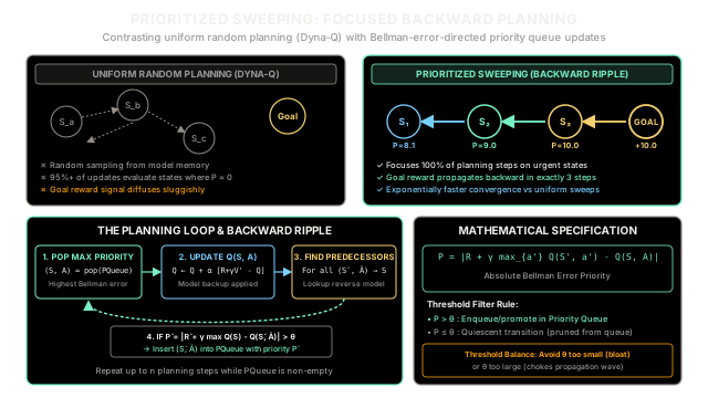
In model-based reinforcement learning, planning algorithms simulate experiences from an environmental model to accelerate value convergence without demanding expensive real-world interactions. In classical architectures like Dyna-Q, simulated transitions are chosen by uniform random sampling over all previously experienced state-action pairs.

In environments with non-trivial state spaces, uniform random planning becomes catastrophically inefficient:

Wasted Computation on Quiescent States: In a maze or gridworld with hundreds of states, 95% or more of state transitions have zero Bellman error—their values are already consistent with their successors. Uniform sampling blindly wastes precious planning cycles computing updates where $\delta = 0.0$ .
Sluggish Diffusion of Goal Surprises: When an agent first stumbles upon a large reward at a goal state, that information must propagate back to the start state. Under uniform sampling, the probability that the model randomly selects the state immediately preceding the goal is small. The probability that it subsequently selects the state two steps prior is smaller still. Propagating a goal signal across $k$ steps requires on the order of $\mathcal{O}(|\mathcal{S}|^k)$ random simulated steps.

Why update transitions at random when we know exactly which states changed?

Introduced independently by Andrew Moore and Christopher Atkeson (1993) and by Jing Peng and Ronald Leisenring (1996), Prioritized Sweeping replaces blind uniform sampling with a priority queue ordered by Bellman error magnitude:

$P = \left| R + \gamma \max_{a'} Q(S', a') - Q(S, A) \right|$

When a major reward or unexpected transition occurs, the algorithm inserts the affected state-action pair into the priority queue. During planning, it pops the highest-priority pair, updates its value, and then works backward: it queries the model for all predecessor state-action pairs that lead into that updated state, computes their anticipated errors, and inserts them into the queue. A single high-impact discovery ripples backward through the state graph directly toward the initial state in a focused wave of updates.

Think of It Like This

Emergency Dispatch Routing in a Major City

Imagine managing an urban emergency response network across hundreds of square miles:

The Dyna-Q Approach (Random Street Patrols): Emergency vehicles randomly patrol suburban cul-de-sacs where nothing has occurred for months. When a massive 5-alarm fire erupts at a chemical plant downtown (a goal reward discovery), dispatch continues telling units to cruise at random. The system hopes that a patrol car will coincidentally wander downtown, notice the fire, and then later wander toward fire stations to notify them. The response is disorganized, diffuse, and painfully slow.
The Prioritized Sweeping Approach (Priority Dispatch Queue): Dispatch maintains an active priority queue sorted strictly by emergency urgency (Bellman error). The chemical plant explosion immediately enters the top of the queue with priority 10.
The Backward Ripple Effect: The moment fire crews respond and contain the epicenter (the goal transition is updated), dispatch does not return to random cruising. It immediately looks up the predecessor arterial avenues and highway exits feeding into downtown (predecessor states). Because traffic is backing up, those feeder junctions are assigned high priority (priority 9.0) and emergency units are routed there next.
Once those arteries are stabilized, the outer ring-roads feeding them receive priority 8.1. The coordination ripples backward along the logistical transport chain directly to where commuters depart, while quiet residential neighborhoods remain untouched.

Where the analogy breaks down: Urban traffic involves continuous fluid dynamics, whereas Prioritized Sweeping operates over discrete Markov transition graphs with explicit predecessor maps. Furthermore, in Prioritized Sweeping, if an update falls below a numerical threshold $\theta$ , it is completely discarded from the queue, whereas emergency dispatch must eventually attend to minor calls.

How It Actually Works

Priority Queue Planning and Backward Ripple Dynamics

Prioritized Sweeping combines an empirical transition model with a max-priority queue (typically implemented with a binary heap) to drive value iteration updates:

1. The Model and Predecessor Graph

The agent maintains two lookup tables based on real-world transitions $(S_t, A_t, R_{t+1}, S_{t+1})$ :

Forward Model: Stores deterministic or expected transitions: $Model(S, A) \to (R, S')$
Predecessor Registry: Maps every successor state $s'$ to the set of state-action pairs that have historically led to it: $Pred(S') = \left\{ (S, A) \mid Model(S, A) \text{ transitions to } S' \right\}$

2. The Priority Metric

The priority $P$ of any state-action pair $(S, A)$ is the absolute magnitude of its one-step Bellman error:

$P \doteq \left| R + \gamma \max_{a'} Q(S', a') - Q(S, A) \right|$

where:

$\gamma \in [0, 1]$ is the discount factor.
$Q(S, A)$ is the current action-value estimate.
$R$ and $S'$ are the predicted reward and next state from $Model(S, A)$ .

If $P > \theta$ (where $\theta > 0$ is a small positive threshold), $(S, A)$ is inserted into the priority queue with priority $P$ . If $(S, A)$ already resides in the queue, its priority is increased to $\max(P_{\text{old}}, P)$ .

3. The Planning Loop

After taking a real step, the agent performs up to $n$ planning iterations while the priority queue is non-empty:

Pop the Top Priority: Remove $(S, A)$ with the largest priority $P$ from the queue: $(S, A) \leftarrow \text{pop\_max}(PQueue)$
Execute Model Backup: Retrieve $(R, S') = Model(S, A)$ and update its action-value: $Q(S, A) \leftarrow Q(S, A) + \alpha \left[ R + \gamma \max_{a'} Q(S', a') - Q(S, A) \right]$ (In deterministic environments, setting $\alpha = 1.0$ sets $Q(S, A)$ exactly to its updated target, reducing its Bellman error to zero).
Propagate Backward to Predecessors: For every predecessor pair $(\bar{S}, \bar{A}) \in Pred(S)$ $(\overset{ˉ}{S}, \overset{ˉ}{A}) \in P r e d (S)$ known to transition into $S$ $S$ :
- Retrieve its predicted reward $\bar{R}$ from $Model(\bar{S}, \bar{A})$ .
- Compute the anticipated Bellman error for the predecessor: $\bar{P} \doteq \left| \bar{R} + \gamma \max_a Q(S, a) - Q(\bar{S}, \bar{A}) \right|$
- If $\bar{P} > \theta$ , insert or promote $(\bar{S}, \bar{A})$ in the priority queue with priority $\bar{P}$ .

4. Quiescence and Convergence

Unlike Dyna-Q, which always runs exactly $n$ simulated steps regardless of whether they are needed, Prioritized Sweeping terminates early if the priority queue becomes empty. When all errors in the network drop below threshold $\theta$ , planning stops naturally, saving computational cycles until another surprise occurs.

Worked numerical example

Consider a 3-state linear chain leading to a terminal goal state:

$S_1 \xrightarrow{\text{right}} S_2 \xrightarrow{\text{right}} S_3 \xrightarrow{\text{right}} S_4 (\text{Goal})$

System Parameters

Discount factor: $\gamma = 0.9$
Step size: $\alpha = 1.0$ (full Bellman backup)
Priority threshold: $\theta = 0.01$
Planning capacity: $n = 10$ steps

Model State

The agent has already traversed $S_1 \to S_2$ and $S_2 \to S_3$ with zero reward, establishing the model and predecessor registry:

$Model(S_1, \text{right}) = (0.0, S_2) \implies Pred(S_2) = \{(S_1, \text{right})\}$
$Model(S_2, \text{right}) = (0.0, S_3) \implies Pred(S_3) = \{(S_2, \text{right})\}$
Initial values: $Q(S_1, \text{right}) = 0.0, Q(S_2, \text{right}) = 0.0, Q(S_3, \text{right}) = 0.0$ .
Terminal state $S_4$ has $\max_a Q(S_4, a) = 0.0$ .

Event: Goal Discovery at $S_3$

The agent executes $(S_3, \text{right})$ , observes reward $R = +10.0$ , and reaches terminal state $S_4$ .

Model Update: $Model(S_3, \text{right}) = (10.0, S_4)$ and $Pred(S_4) = \{(S_3, \text{right})\}$ .
Initial Bellman Error: $P = |10.0 + 0.9 \times 0.0 - 0.0| = 10.0000$
Queue Insertion: Because $10.0 > 0.01$ , insert $(S_3, \text{right})$ into $PQueue$ with priority $P = 10.0000$ .

Planning Iteration 1

Pop: Top element is $(S_3, \text{right})$ with priority $10.0000$ .
Update $Q(S_3, \text{right})$ : $Q(S_3, \text{right}) \leftarrow 0.0 + 1.0 \times [10.0 + 0.9 \times 0.0 - 0.0] = 10.0000$
Backward Lookup: Predecessors of $S_3$ $S_{3}$ is $Pred(S_3) = \{(S_2, \text{right})\}$ $P r e d (S_{3}) = {(S_{2}, right)}$ .
- For $(S_2, \text{right})$ , predicted reward is $\bar{R} = 0.0$ and next state is $S_3$ .
- Compute predecessor priority: $\bar{P} = |0.0 + 0.9 \times \max Q(S_3) - Q(S_2, \text{right})| = |0.0 + 0.9 \times 10.0 - 0.0| = 9.0000$
- Since $9.0000 > 0.01$ , insert $(S_2, \text{right})$ into $PQueue$ with priority $9.0000$ .

Planning Iteration 2

Pop: Top element is $(S_2, \text{right})$ with priority $9.0000$ .
Update $Q(S_2, \text{right})$ : $Q(S_2, \text{right}) \leftarrow 0.0 + 1.0 \times [0.0 + 0.9 \times 10.0 - 0.0] = 9.0000$
Backward Lookup: Predecessors of $S_2$ $S_{2}$ is $Pred(S_2) = \{(S_1, \text{right})\}$ $P r e d (S_{2}) = {(S_{1}, right)}$ .
- For $(S_1, \text{right})$ , predicted reward is $\bar{R} = 0.0$ and next state is $S_2$ .
- Compute predecessor priority: $\bar{P} = |0.0 + 0.9 \times \max Q(S_2) - Q(S_1, \text{right})| = |0.0 + 0.9 \times 9.0 - 0.0| = 8.1000$
- Since $8.1000 > 0.01$ , insert $(S_1, \text{right})$ into $PQueue$ with priority $8.1000$ .

Planning Iteration 3

Pop: Top element is $(S_1, \text{right})$ with priority $8.1000$ .
Update $Q(S_1, \text{right})$ : $Q(S_1, \text{right}) \leftarrow 0.0 + 1.0 \times [0.0 + 0.9 \times 9.0 - 0.0] = 8.1000$
Backward Lookup: $S_1$ has no predecessors ( $Pred(S_1) = \emptyset$ ).
Queue Status: The priority queue is now empty. Planning terminates after exactly 3 steps.

Result Comparison

In just 3 focused planning steps, the goal reward rippled completely across the 3-state chain:

$Q(S_3, \text{right}) = 10.0000$
$Q(S_2, \text{right}) = 9.0000$
$Q(S_1, \text{right}) = 8.1000$

Under uniform random Dyna-Q with 100 transitions in memory, achieving this backward cascade would have required hundreds of exploratory iterations.

Code

Below is a complete, type-hinted Python implementation of Prioritized Sweeping utilizing a priority queue built on Python's standard heapq module:

1import heapq2from typing import Dict, List, Optional, Set, Tuple3
4
5class PriorityQueue:6    """Max-priority queue wrapper using heapq supporting priority promotion."""7
8    def __init__(self) -> None:9        self._heap: List[Tuple[float, int, Optional[Tuple[str, str]]]] = []10        self._entry_finder: Dict[Tuple[str, str], List] = {}11        self._counter: int = 012
13    def push_or_update(self, item: Tuple[str, str], priority: float) -> None:14        """Insert or increase priority of an existing state-action pair."""15        if item in self._entry_finder:16            existing_entry = self._entry_finder[item]17            existing_priority = -existing_entry[0]18            # In prioritized sweeping, retain the higher priority19            if priority <= existing_priority:20                return21            # Invalidate older entry in heap22            existing_entry[-1] = None23
24        self._counter += 125        # Store negative priority because heapq implements a min-heap26        entry = [-priority, self._counter, item]27        self._entry_finder[item] = entry28        heapq.heappush(self._heap, entry)29
30    def pop(self) -> Tuple[Tuple[str, str], float]:31        """Pop and return (item, priority) with the highest priority."""32        while self._heap:33            neg_pri, _, item = heapq.heappop(self._heap)34            if item is not None:35                del self._entry_finder[item]36                return item, -neg_pri37        raise IndexError("Cannot pop from an empty PriorityQueue")38
39    def __bool__(self) -> bool:40        return bool(self._entry_finder)41
42    def __len__(self) -> int:43        return len(self._entry_finder)44
45
46class PrioritizedSweeping:47    """Model-based Prioritized Sweeping algorithm."""48
49    def __init__(50        self,51        states: List[str],52        actions: List[str],53        gamma: float = 0.9,54        alpha: float = 1.0,55        theta: float = 0.01,56        max_planning_steps: int = 10,57    ) -> None:58        self.states = states59        self.actions = actions60        self.gamma = gamma61        self.alpha = alpha62        self.theta = theta63        self.max_planning_steps = max_planning_steps64
65        # Action-value table66        self.q: Dict[Tuple[str, str], float] = {67            (s, a): 0.0 for s in states for a in actions68        }69
70        # Transition model: (state, action) -> (reward, next_state)71        self.model: Dict[Tuple[str, str], Tuple[float, str]] = {}72
73        # Reverse predecessor index: state -> set of (pred_state, pred_action)74        self.predecessors: Dict[str, Set[Tuple[str, str]]] = {75            s: set() for s in states76        }77
78        self.pqueue = PriorityQueue()79
80    def get_max_q(self, state: str) -> float:81        """Return max_a Q(state, a) or 0.0 if state is terminal."""82        q_vals = [self.q[(state, a)] for a in self.actions if (state, a) in self.q]83        return max(q_vals) if q_vals else 0.084
85    def step(86        self,87        state: str,88        action: str,89        reward: float,90        next_state: str,91        is_terminal: bool = False,92    ) -> List[Tuple[Tuple[str, str], float, float]]:93        """Process an experience transition and perform prioritized planning.94
95        Returns:96            List of planning steps: [((state, action), priority, new_q_value), ...]97        """98        # 1. Update learned model and predecessor graph99        self.model[(state, action)] = (reward, next_state)100        if next_state not in self.predecessors:101            self.predecessors[next_state] = set()102        self.predecessors[next_state].add((state, action))103
104        # 2. Compute Bellman error for experienced transition105        next_max = 0.0 if is_terminal else self.get_max_q(next_state)106        target = reward + self.gamma * next_max107        priority = abs(target - self.q[(state, action)])108
109        # 3. Insert into queue if priority exceeds threshold110        if priority > self.theta:111            self.pqueue.push_or_update((state, action), priority)112
113        # 4. Backward planning ripple loop114        planning_trace: List[Tuple[Tuple[str, str], float, float]] = []115        steps_executed = 0116
117        while self.pqueue and steps_executed < self.max_planning_steps:118            steps_executed += 1119            (s, a), popped_p = self.pqueue.pop()120
121            r, s_next = self.model[(s, a)]122            s_next_max = 0.0 if (s_next == "S4" or is_terminal) else self.get_max_q(s_next)123            td_target = r + self.gamma * s_next_max124            self.q[(s, a)] += self.alpha * (td_target - self.q[(s, a)])125            planning_trace.append(((s, a), popped_p, self.q[(s, a)]))126
127            # Backward ripple: inspect all predecessors that lead into s128            for s_bar, a_bar in self.predecessors.get(s, set()):129                r_bar, _ = self.model[(s_bar, a_bar)]130                pred_target = r_bar + self.gamma * self.get_max_q(s)131                pred_p = abs(pred_target - self.q[(s_bar, a_bar)])132                if pred_p > self.theta:133                    self.pqueue.push_or_update((s_bar, a_bar), pred_p)134
135        return planning_trace136
137
138def demonstrate_prioritized_sweeping() -> None:139    states = ["S1", "S2", "S3", "S4"]140    actions = ["right"]141    ps = PrioritizedSweeping(142        states, actions, gamma=0.9, alpha=1.0, theta=0.01, max_planning_steps=10143    )144
145    # Pre-populate model with known transitions leading toward goal146    ps.model[("S1", "right")] = (0.0, "S2")147    ps.predecessors["S2"].add(("S1", "right"))148    ps.model[("S2", "right")] = (0.0, "S3")149    ps.predecessors["S3"].add(("S2", "right"))150
151    print("--- Experiencing Goal Discovery: S3 -> S4 with R=+10.0 ---")152    trace = ps.step("S3", "right", 10.0, "S4", is_terminal=True)153    for step_num, ((s, a), p, new_val) in enumerate(trace, 1):154        print(155            f"Planning Step {step_num}: Popped ({s}, {a}) with priority {p:.4f} "156            f"-> Q updated to {new_val:.4f}"157        )158
159    print("\n--- Final Q-Values after Backward Ripple ---")160    for s in ["S1", "S2", "S3"]:161        print(f"Q({s}, right) = {ps.q[(s, 'right')]:.4f}")162
163    assert abs(ps.q[("S3", "right")] - 10.0) < 1e-4164    assert abs(ps.q[("S2", "right")] - 9.0) < 1e-4165    assert abs(ps.q[("S1", "right")] - 8.1) < 1e-4166
167
168if __name__ == "__main__":169    demonstrate_prioritized_sweeping()170
171# -> Expected output:172# -> --- Experiencing Goal Discovery: S3 -> S4 with R=+10.0 ---173# -> Planning Step 1: Popped (S3, right) with priority 10.0000 -> Q updated to 10.0000174# -> Planning Step 2: Popped (S2, right) with priority 9.0000 -> Q updated to 9.0000175# -> Planning Step 3: Popped (S1, right) with priority 8.1000 -> Q updated to 8.1000176# -> 177# -> --- Final Q-Values after Backward Ripple ---178# -> Q(S1, right) = 8.1000179# -> Q(S2, right) = 9.0000180# -> Q(S3, right) = 10.0000

Watch Out For

The Threshold Tuning Dilemma: Queue Explosion vs. Frozen Planning

The priority threshold $\theta$ dictates the boundary between urgent updates and ignorable noise. Choosing an inappropriate $\theta$ causes severe systemic failures:

The Symptom:

Queue Thrashing ( $\theta$ too small): In stochastic environments or dense transition graphs, setting $\theta \approx 0$ causes thousands of minuscule numerical adjustments to enter the heap. Heap management overhead ( $\mathcal{O}(\log |Q|)$ per insertion) quickly dominates total wall-clock runtime, consuming more CPU cycles than environmental interaction itself.
Frozen Propagation ( $\theta$ too large): If $\theta$ is set too high relative to reward magnitudes, the backward ripple wave prematurely attenuates. Because predecessor errors decay geometrically by $\gamma$ ( $\bar{P} \propto \gamma^k P$ ), a high threshold stops the value wave after just one or two steps, leaving distant start states completely unaware of discovered goals.

The Fix:

Scale $\theta$ proportionally to the environment's reward magnitude and discount factor: a practical rule of thumb is $\theta \approx 10^{-3} \times |R_{\max} - R_{\min}|$ .
Always enforce an explicit cap on planning steps per real interaction (max_planning_steps = n). This bounds computation per environmental step regardless of queue size.
In stochastic environments, maintain expected transition probability models $\sum_{s'} p(s' \mid s, a)$ rather than deterministic overwrites to prevent stochastic transition jitter from triggering phantom priority spikes.

The Quick Version

Urgency-Driven Planning: Prioritized sweeping replaces Dyna-Q's blind uniform sampling with a priority queue ordered by absolute Bellman error $P = |R + \gamma \max Q(S') - Q(S, A)|$ .
Backward Value Propagation: Whenever a high-priority state is updated, the algorithm inspects all predecessor transitions that lead into it, queuing them to receive the newly computed value signal.
Exponentially Faster Learning: High-magnitude discoveries ripple backward toward the starting state in a direct cascade, reducing the number of planning steps required for goal information to propagate by orders of magnitude.
Threshold Controlled: The priority threshold $\theta$ acts as a filter, pruning quiescent transitions from the queue to prevent wasted computation on states whose values have already converged.