Planning and Learning

Learning improves decisions through direct trial-and-error in the real world, while planning mentally simulates prospective scenarios using an internal model. Combining both enables rapid learning without risking costly real-world mistakes.

Why Does This Exist?

In classic reinforcement learning, algorithms are often split into two seemingly disconnected paradigms:

Model-free learning: The agent takes physical actions in the real environment, observes rewards, and updates its value estimates through direct trial-and-error (e.g., Q-learning or SARSA).
Model-based planning: The agent possesses an explicit model of transition dynamics and rewards, computing optimal policies through forward search or state-space sweeps (e.g., Dynamic Programming or Monte Carlo Tree Search).

In physical domains—such as robotics, autonomous driving, or industrial process automation—relying purely on real-world trial-and-error is prohibitively expensive, agonizingly slow, and physically dangerous. An autonomous car cannot afford to crash into barriers hundreds of times just to learn that collisions carry a negative reward.

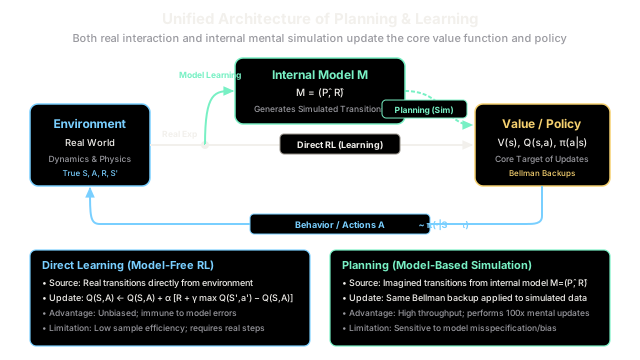
The unified framework of planning and learning solves this fundamental bottleneck. It reveals that learning and planning are not mutually exclusive alternatives; they are complementary processes operating on the exact same core currency: Bellman value updates. By integrating both into a unified closed loop, real experience is used both to update values immediately and to learn an internal predictive model of the environment. That model then generates synthetic transitions to update policies hundreds of times faster than real time permits.

Think of It Like This

The Grandmaster's Mental Simulation

Imagine a world-class chess grandmaster competing in a high-stakes championship tournament.

When it is the grandmaster's turn:

Real Experience: She reaches out, picks up a rook, and places it on square e4. She presses the clock. That single physical move is an interaction with the external environment. She observes her opponent's real reaction and face-to-face clock pressure.
Mental Planning: As her opponent deliberates, the grandmaster does not sit with an empty mind waiting for the next turn. She closes her eyes and simulates ten moves ahead in her imagination: "If he moves the bishop to f5, I strike with knight to d5; if he pushes the c-pawn, I castle queenside."

None of those imagined board states are physically placed on the wooden table, yet every mental rehearsal updates her internal evaluation of which board formations are advantageous. When her opponent finally moves, she already knows the winning response because she has already experienced it dozens of times in her head.

Where the analogy stops: Human grandmasters simulate complex, deep tree structures with tactical pruning and heuristic pattern recognition. In computational reinforcement learning, planning often takes the form of randomized state-action background replays drawn from a learned lookup model or parametric neural network. Furthermore, if the grandmaster's mental model misremembers the rules of piece movement, her imaginary simulations will teach her disastrous blunders.

How It Actually Works

The Shared Foundation: Bellman Updates

At the heart of the unified perspective lies a profound insight formulated by Richard Sutton: planning and learning use the exact same mathematical updates to modify value functions and policies.

Both paradigms estimate state values $V(s)$ or action values $Q(s, a)$ by applying Bellman backups. For instance, in Q-learning:

$Q(S, A) \leftarrow Q(S, A) + \alpha \left[ R + \gamma \max_{a'} Q(S', a') - Q(S, A) \right]$

The only difference between learning and planning is the origin of the transition quadruple $(S, A, R, S')$ :

Learning (Model-Free RL): The transition $(S_t, A_t, R_{t+1}, S_{t+1})$ is generated by the real external environment.
Planning (Model-Based RL): The transition $(S, A, R, S')$ is generated by an internal environment model $\mathcal{M}$ .

Internal Models: Sample Models vs. Distribution Models

An internal model $\mathcal{M}$ is any computational process that mimics environmental dynamics. Given a state $S$ and action $A$ , a model predicts possible future outcomes:

Distribution Models: A distribution model produces the complete probability distribution over all possible next states and expected rewards: $\mathcal{M}_{\text{dist}} = \{P(s' \mid s, a), \; R(s, a, s')\}$ Planning method: Exhaustive expected Bellman backups, as performed in classic Dynamic Programming. While mathematically rigorous, distribution models require massive memory and cannot be sampled cheaply in high-dimensional or continuous state spaces.
Sample Models: A sample model acts as an internal simulator. Given current state $S$ and chosen action $A$ , it draws a single concrete sample according to underlying transition probabilities: $(R, S') \sim \mathcal{M}_{\text{sample}}(S, A)$ Planning method: Sample backups and simulated rollouts, identical in format to real experience. Sample models can be queried cheaply and parallelized effortlessly on modern hardware.

The Unified Feedback Architecture (Dyna)

The synthesis of planning, acting, and model learning forms the canonical Dyna architecture:

1                       +-------------------+2                       |    Environment    |3                       +-------------------+4                         ^               |5                 Action  |               | Real Experience6                   A_t   |               | (S_t, A_t, R_{t+1}, S_{t+1})7                         |               v8                   +-----------+   +-----------+9                   |  Policy / |<--|   Model   |10                   |   Value   |   |  Learning |11                   +-----------+   +-----------+12                         ^               |13                         |               | Internal Model M = (P_hat, R_hat)14                         |               v15                         |      +-----------------+16                         +------|    Planning     |17                     Simulated  | (Simulated Exp) |18                      Backups   +-----------------+

On every time step:

Act: The agent selects action $A_t \sim \pi(\cdot \mid S_t)$ based on its current value function and executes it in the real environment.
Direct RL: The real transition $(S_t, A_t, R_{t+1}, S_{t+1})$ updates the value function directly via a standard TD backup.
Model Learning: The real transition updates the internal model $\mathcal{M} = (\hat{P}, \hat{R})$ to better approximate real-world physics.
Planning: The agent pauses its physical actions and executes $N$ $N$ simulated planning steps:
- Sample previously visited state-action pair $(S_k, A_k)$ .
- Query model: $(R_k, S'_k) \leftarrow \mathcal{M}(S_k, A_k)$ .
- Apply standard Bellman backup to $Q(S_k, A_k)$ using the simulated outcome.

Worked numerical comparison of convergence speed

Consider a linear corridor task with three states $\{S_0, S_1, S_2\}$ , where $S_2$ is a rewarding terminal goal: $S_0 \xrightarrow{\text{Forward}} S_1 \xrightarrow{\text{Forward}} S_2 \quad (\text{Goal Reward } R = 10.0)$

Hyperparameters:

Initial action values: $Q(S_0) = 0.0, \; Q(S_1) = 0.0, \; Q(S_2) = 0.0$ .
Step size $\alpha = 0.5$ , discount factor $\gamma = 0.9$ .

Case 1: Pure Direct RL (No Planning, $N=0$ )

Step 0: Agent executes $(S_0, \text{Forward}) \to S_1$ with reward $R_1 = 0$ . $Q(S_0) \leftarrow Q(S_0) + 0.5 \left[ 0 + 0.9 Q(S_1) - Q(S_0) \right] = 0.0 + 0.5[0 + 0 - 0] = \mathbf{0.0}$
Step 1: Agent executes $(S_1, \text{Forward}) \to S_2$ with reward $R_2 = 10.0$ . $Q(S_1) \leftarrow Q(S_1) + 0.5 \left[ 10.0 + 0.9(0) - Q(S_1) \right] = 0.0 + 0.5[10.0 - 0] = \mathbf{5.0}$
Result at episode end: $Q(S_1) = 5.0$ , but $Q(S_0) = \mathbf{0.0}$ . The start state learned nothing about the goal during this entire episode. Information requires a second physical episode to propagate back to $S_0$ .

Case 2: Integrated Planning & Learning ( $N=2$ Planning Steps)

Step 0: Real transition $S_0 \to S_1, R=0$ . Direct RL updates $Q(S_0) = 0.0$ . Model stores $\mathcal{M}(S_0) = (S_1, 0)$ .
Step 1: Real transition $S_1 \to S_2, R=10.0$ . Direct RL updates $Q(S_1) = \mathbf{5.0}$ . Model stores $\mathcal{M}(S_1) = (S_2, 10.0)$ .
Immediate Planning Phase (mental simulation):
- Planning Step 1: Query model for state $S_1$ : $\mathcal{M}(S_1) = (S_2, 10.0)$ . $Q(S_1) \leftarrow 5.0 + 0.5 [10.0 + 0 - 5.0] = \mathbf{7.5}$
- Planning Step 2: Query model for state $S_0$ : $\mathcal{M}(S_0) = (S_1, 0.0)$ . $Q(S_0) \leftarrow 0.0 + 0.5 \left[ 0.0 + 0.9 Q(S_1) - 0.0 \right] = 0.5 [0.9 \times 7.5] = \mathbf{3.375}$

In the exact same physical episode, the integrated planning agent propagated goal information all the way back to the initial start state $S_0$ ( $Q(S_0) = 3.375$ vs. $0.0$ ), saving real-world exploration time.

Code

1import random2from typing import Dict, List, Tuple3
4
5def step_environment(state: int, action: str) -> Tuple[int, float]:6    """Simulate a 5-state grid corridor (0: start -> 4: terminal goal)."""7    if action == "right":8        next_state = min(state + 1, 4)9    else:10        next_state = max(state - 1, 0)11    reward = 10.0 if next_state == 4 else 0.012    return next_state, reward13
14
15def evaluate_planning_vs_learning(16    num_episodes: int = 5,17    planning_steps: int = 5,18    alpha: float = 0.5,19    gamma: float = 0.9,20    seed: int = 42,21) -> Tuple[float, float]:22    """Compare pure Direct Q-learning against Dyna-style Integrated Planning & Learning.23
24    Args:25        num_episodes: Number of training episodes.26        planning_steps: Number of simulated planning updates per real step.27        alpha: Learning rate step size.28        gamma: Discount factor.29        seed: Random seed for deterministic reproducibility.30
31    Returns:32        Tuple of (direct_rl_start_q, integrated_planning_start_q).33    """34    states = [0, 1, 2, 3, 4]35    actions = ["left", "right"]36
37    # -------------------------------------------------------------38    # 1. Pure Direct RL (Model-Free Q-learning, N = 0 planning steps)39    # -------------------------------------------------------------40    random.seed(seed)41    q_direct: Dict[Tuple[int, str], float] = {42        (s, a): 0.0 for s in states for a in actions43    }44
45    for ep in range(num_episodes):46        s = 047        while s != 4:48            a = "right" if random.random() < 0.8 else "left"49            next_s, r = step_environment(s, a)50            best_next_q = (51                max(q_direct[(next_s, act)] for act in actions)52                if next_s != 453                else 0.054            )55            td_target = r + gamma * best_next_q56            q_direct[(s, a)] += alpha * (td_target - q_direct[(s, a)])57            s = next_s58
59    # -------------------------------------------------------------60    # 2. Integrated Planning and Learning (Dyna-Q with N planning steps)61    # -------------------------------------------------------------62    random.seed(seed)63    q_plan: Dict[Tuple[int, str], float] = {64        (s, a): 0.0 for s in states for a in actions65    }66    model: Dict[Tuple[int, str], Tuple[int, float]] = {}67
68    for ep in range(num_episodes):69        s = 070        while s != 4:71            a = "right" if random.random() < 0.8 else "left"72            next_s, r = step_environment(s, a)73
74            # A. Direct RL update from real experience75            best_next_q = (76                max(q_plan[(next_s, act)] for act in actions)77                if next_s != 478                else 0.079            )80            q_plan[(s, a)] += alpha * (r + gamma * best_next_q - q_plan[(s, a)])81
82            # B. Model learning: store observed deterministic transition83            model[(s, a)] = (next_s, r)84
85            # C. Planning: perform N simulated updates from internal model86            for _ in range(planning_steps):87                sim_s, sim_a = random.choice(list(model.keys()))88                sim_next, sim_r = model[(sim_s, sim_a)]89                best_sim_next_q = (90                    max(q_plan[(sim_next, act)] for act in actions)91                    if sim_next != 492                    else 0.093                )94                q_plan[(sim_s, sim_a)] += alpha * (95                    sim_r + gamma * best_sim_next_q - q_plan[(sim_s, sim_a)]96                )97
98            s = next_s99
100    q_direct_start = q_direct[(0, "right")]101    q_plan_start = q_plan[(0, "right")]102    return q_direct_start, q_plan_start103
104
105if __name__ == "__main__":106    direct_val, plan_val = evaluate_planning_vs_learning(107        num_episodes=5, planning_steps=5108    )109
110    print("=== Convergence Comparison at Start State Q(0, 'right') ===")111    print(f"Direct RL (N=0) Value:        {direct_val:.4f}")112    print(f"Integrated Planning (N=5) Value: {plan_val:.4f}")113
114    # Assertion confirming planning drastically accelerates value propagation115    assert (116        plan_val > direct_val117    ), "Planning must accelerate credit assignment back to start state!"118    print(119        f"\nValidation passed: Planning accelerated value propagation by {plan_val / direct_val:.2f}x."120    )121
122# Expected Output:123# === Convergence Comparison at Start State Q(0, 'right') ===124# Direct RL (N=0) Value:        1.8225125# Integrated Planning (N=5) Value: 7.2896126#127# Validation passed: Planning accelerated value propagation by 4.00x.

Watch Out For

Compounding Model Bias and Hallucinated Planning Updates

The central vulnerability of planning is that the value function converges to the optimal policy for the learned internal model, which may diverge sharply from the real environment.

When an internal model is trained on limited data, is overparameterized, or encounters non-stationary dynamics, it develops subtle prediction biases. Because planning iterates simulated updates repeatedly through this flawed model, initial small errors compound exponentially across imaginary rollout steps:

The agent uncovers "phantom rewards" or hallucinated shortcuts that do not exist in physical reality.
The policy overfits to model artifacts, resulting in catastrophic failure when tested back in the real world.

The Fix:

Dyna-Q+ Exploration Bonuses: Reward the agent with an exploration bonus ( $\kappa \sqrt{\tau}$ ) for visiting state-action pairs that have not been tested in real life for $\tau$ steps, actively keeping the internal model fresh.
Short Planning Horizons: Limit simulated rollouts to short horizons ( $k \in [1, 5]$ steps) rather than full imaginary episodes, constraining accumulated transition error (e.g., Model-Based Policy Optimization / MBPO).
Ensemble Models: Maintain an ensemble of models and plan only over transitions where ensemble disagreement is low (uncertainty-aware planning).

The Quick Version

Shared algorithmic currency: Both learning and planning update state-action values using the identical Bellman equation; they differ solely in whether transitions originate from the real environment or an internal simulator.
The Dyna feedback loop: Real experience serves a dual purpose: it updates the value function directly (Direct RL) and trains the internal environment model $\mathcal{M} = (\hat{P}, \hat{R})$ .
Sample vs. distribution models: Distribution models describe complete probability distributions for exhaustive DP sweeps; sample models draw concrete transitions, enabling fast, parallelized Monte Carlo planning.
Sample efficiency vs. model bias: Planning dramatically reduces the number of physical real-world interactions required to learn, but risks policy failure if the internal model develops compounding simulation errors.