Emphatic-TD Methods in RL

Emphatic-TD stabilizes off-policy learning by re-weighting updates with followon traces, ensuring errors in frequently bootstrapped states are corrected before they cause divergence.

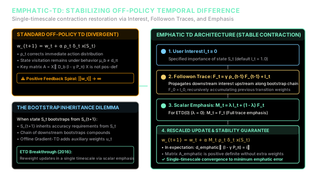
Emphatic-TD dynamically scales semi-gradient updates via interest and followon traces, restoring positive definiteness to off-policy learning.

Why Does This Exist?

In reinforcement learning, the Deadly Triad—combining function approximation, bootstrapping, and off-policy data—causes standard temporal-difference algorithms to diverge. In standard off-policy $\text{TD}(0)$ , weighting updates with the importance sampling ratio $\rho_t = \frac{\pi(A_t|S_t)}{b(A_t|S_t)}$ corrects for the discrepancy in action selection probabilities, but it does nothing to correct the underlying state distribution mismatch. Transitions remain sampled according to the behavior policy's visitation frequency $\mu_b$ rather than the target policy's stationary distribution $d_\pi$ .

Because $\mu_b \neq d_\pi$ , the expected update matrix:

$\mathbf{A}_{\text{off}} = \mathbf{X}^\top \mathbf{D}_b (\mathbf{I} - \gamma \mathbf{P}_\pi) \mathbf{X}$

is not guaranteed to have a positive-definite symmetric part. When $\mathbf{A}_{\text{off}}$ develops eigenvalues with negative real parts, the spectral radius of the iteration matrix exceeds unity ( $\rho(\mathbf{I} - \alpha \mathbf{A}_{\text{off}}) > 1$ ). This creates an unstable positive feedback loop where value estimates grow exponentially to $\pm \infty$ .

Historically, the primary remedy was Gradient-TD (such as TDC and GTD2). Gradient-TD converts policy evaluation into a saddle-point optimization problem minimizing the Mean Squared Projected Bellman Error (MSPBE). However, Gradient-TD requires:

An auxiliary secondary weight vector $\mathbf{u}_t \in \mathbb{R}^d$ running alongside $\mathbf{w}_t$ .
Two separate learning rates ( $\alpha_t$ and $\beta_t$ ) operating on two distinct timescales ( $\beta_t / \alpha_t \to 0$ ), which makes hyperparameter tuning delicate and empirical convergence sluggish.

In 2016, Richard Sutton, A. Rupam Mahmood, and Martha White introduced Emphatic Temporal-Difference (ETD) learning. Rather than minimizing a dual projected objective with two timescales, ETD solves the problem directly within a single timescale using a single weight vector $\mathbf{w}_t$ and one learning rate $\alpha$ . By recursively tracking how downstream states inherit bootstrapping obligations through a scalar followon trace, ETD re-weights updates with an emphasis scalar $M_t$ . This reshapes the effective state distribution such that the resulting system matrix is provably positive definite, restoring contraction and stability to off-policy semi-gradient learning.

Think of It Like This

The Audio Feedback Compressor

Imagine a live performance sound system with high-gain microphones and loud stage monitors. When sound emitted by a monitor leaks back into a microphone, it creates a closed acoustic loop. If certain resonant frequencies circulate unchecked, the amplifier boosts them on every pass, culminating in an ear-piercing screech of acoustic feedback. This runaway screech is the exact physical analogue of the Deadly Triad.

The Gradient-TD solution is like placing a second, independent digital signal processor (DSP) in the audio rack. The secondary processor runs its own background phase-cancellation algorithm on a slower internal clock, calculating a continuous anti-feedback curve and subtracting it from the primary audio stream. It stops the feedback, but it doubles hardware complexity and introduces latency.

Emphatic-TD, by contrast, is an adaptive feedback compressor built directly into the main audio channel. It maintains a running memory of recent signal surges (the followon trace $F_t$ ). Whenever the performer hits a note that previously leaked into the monitor and caused an amplification spike downstream, the compressor dynamically modulates channel gain (the emphasis $M_t$ ) right at that moment. By attenuating resonant peaks and elevating damped passages, the net loop gain across all frequencies stays strictly below unity. The system achieves maximum amplification without screeching, without auxiliary secondary processors.

Where the analogy stops: An audio compressor only reduces signal gain to prevent clipping. Emphatic-TD can dynamically both amplify and attenuate updates—boosting states whose downstream predictions are heavily relied upon, and damping unvisited states—to ensure the mathematical operator strictly contracts in expectation.

How It Actually Works

Followon Traces, Emphasis, and the Emphatic Matrix

Emphatic-TD introduces three interconnected quantities that propagate bootstrapping importance:

User Interest ( $I_t \ge 0$ ): A user-specified scalar defining how much the practitioner cares about prediction accuracy in state $S_t$ . In standard uniform policy evaluation, $I_t = 1.0$ for all states. In selective evaluation (e.g., predicting value only for sub-tasks or start states), $I_t$ can be set to $1.0$ on target states and $0.0$ elsewhere.
The Followon Trace ( $F_t$ ): When state $S_t$ bootstraps from future states $S_{t+1}, S_{t+2}, \dots$ , errors in those future states propagate backward to degrade the prediction at $S_t$ . Therefore, any future state that is bootstrapped into inherits interest from the preceding states that relied upon it. The followon trace recursively accumulates this inherited interest forward in time:

$F_0 = I_0$

$F_t = \gamma \rho_{t-1} F_{t-1} + I_t \quad (t \ge 1)$

where $\rho_{t-1} = \frac{\pi(A_{t-1}|S_{t-1})}{b(A_{t-1}|S_{t-1})}$ is the importance sampling ratio of the transition arriving into state $S_t$ , and $\gamma \in [0, 1)$ is the discount factor.
The Emphasis Scalar ( $M_t$ ): The scalar weight applied to the semi-gradient update at time $t$ . For general multi-step $\text{ETD}(\lambda)$ , emphasis balances immediate interest against the accumulated followon trace:

$M_t = \lambda I_t + (1 - \lambda) F_t$

For the fundamental 1-step algorithm ( $\text{ETD}(0)$ , where $\lambda = 0$ ):

$M_t = F_t$

The eligibility trace vector $\mathbf{e}_t \in \mathbb{R}^d$ for $\text{ETD}(\lambda)$ combines the emphasis scalar with state features:

$\mathbf{e}_t = \rho_t \left( \gamma \lambda \mathbf{e}_{t-1} + M_t \mathbf{x}(S_t) \right), \quad \text{with } \mathbf{e}_{-1} = \mathbf{0}$

For $\text{ETD}(0)$ ( $\lambda = 0$ ), this simplifies to:

$\mathbf{e}_t = \rho_t M_t \mathbf{x}(S_t)$

The parameter update rule is:

$\mathbf{w}_{t+1} = \mathbf{w}_t + \alpha \delta_t \mathbf{e}_t = \mathbf{w}_t + \alpha M_t \rho_t \delta_t \mathbf{x}(S_t)$

where $\delta_t = R_{t+1} + \gamma \hat{v}(S_{t+1}, \mathbf{w}_t) - \hat{v}(S_t, \mathbf{w}_t)$ is the standard temporal difference error.

Why Contraction and Stability are Guaranteed

Under behavior policy $b$ , the steady-state expectation of the emphasis vector defines an asymptotic diagonal weighting matrix:

$\mathbf{d}_{\text{emphatic}}^\top = \mathbf{i}^\top (\mathbf{I} - \gamma \mathbf{P}_\pi)^{-1}$

where $\mathbf{i} = [I(s_1), \dots, I(s_n)]^\top$ is the interest vector and $\mathbf{P}_\pi$ is the target policy transition matrix. Post-multiplying both sides by $(\mathbf{I} - \gamma \mathbf{P}_\pi)$ yields:

$\mathbf{d}_{\text{emphatic}}^\top (\mathbf{I} - \gamma \mathbf{P}_\pi) = \mathbf{i}^\top > \mathbf{0}$

Let $\mathbf{D}_{\text{emphatic}} = \text{diag}(\mathbf{d}_{\text{emphatic}})$ . The expected linear system matrix under ETD updates becomes:

$\mathbf{A}_{\text{emphatic}} = \mathbf{X}^\top \mathbf{D}_{\text{emphatic}} (\mathbf{I} - \gamma \mathbf{P}_\pi) \mathbf{X}$

Sutton, Mahmood, and White proved that for any interest vector $\mathbf{i} > \mathbf{0}$ , the symmetric part:

$\frac{1}{2} \left[ \mathbf{D}_{\text{emphatic}} (\mathbf{I} - \gamma \mathbf{P}_\pi) + (\mathbf{I} - \gamma \mathbf{P}_\pi)^\top \mathbf{D}_{\text{emphatic}} \right]$

is strictly positive definite. As a result, $\mathbf{A}_{\text{emphatic}}$ has all eigenvalues with strictly positive real parts, guaranteeing that the ordinary differential equation $\dot{\mathbf{w}} = \mathbf{b}_{\text{emphatic}} - \mathbf{A}_{\text{emphatic}}\mathbf{w}$ is asymptotically stable. $\mathbf{w}_t$ converges to the unique fixed point $\mathbf{w}^* = \mathbf{A}_{\text{emphatic}}^{-1} \mathbf{b}_{\text{emphatic}}$ with probability 1.

Worked numerical example

To observe how the followon trace and emphasis dynamically rescale off-policy updates, consider a two-step trajectory in a 2-state MDP with linear function approximation:

State Features: $\mathbf{x}(s_1) = [1.0, 0.0]^\top$ , $\mathbf{x}(s_2) = [0.0, 2.0]^\top$ .
Parameters: $\mathbf{w}_0 = [1.0, 1.0]^\top$ . Initial value estimates: $\hat{v}(s_1, \mathbf{w}_0) = [1.0, 0.0] \cdot [1.0, 1.0] = 1.0$ $\hat{v}(s_2, \mathbf{w}_0) = [0.0, 2.0] \cdot [1.0, 1.0] = 2.0$
Hyperparameters: $\gamma = 0.9$ , $\alpha = 0.05$ , uniform interest $I_t = 1.0$ , $\lambda = 0$ ( $\text{ETD}(0)$ ). All transition rewards $R = 0.0$ .

Transition 0 ( $t = 0$ ): $S_0 = s_1 \to S_1 = s_2$

Followon Trace and Emphasis: $F_0 = I_0 = 1.0000, \quad M_0 = F_0 = 1.0000$
Action Selection and Importance Ratio: Target takes $a_1$ with $\pi(a_1|s_1) = 1.0$ ; behavior takes $a_1$ with $b(a_1|s_1) = 0.5$ : $\rho_0 = \frac{\pi(a_1|s_1)}{b(a_1|s_1)} = \frac{1.0}{0.5} = 2.0000$
Temporal Difference Error: $\delta_0 = R_1 + \gamma \hat{v}(s_2, \mathbf{w}_0) - \hat{v}(s_1, \mathbf{w}_0) = 0.0 + 0.9(2.0) - 1.0 = 1.8 - 1.0 = +0.8000$
Parameter Update: $\mathbf{w}_1 = \mathbf{w}_0 + \alpha M_0 \rho_0 \delta_0 \mathbf{x}(s_1)$ $\mathbf{w}_1 = \begin{bmatrix} 1.0 \\ 1.0 \end{bmatrix} + 0.05 \times 1.0 \times 2.0 \times 0.8 \times \begin{bmatrix} 1.0 \\ 0.0 \end{bmatrix} = \begin{bmatrix} 1.0 \\ 1.0 \end{bmatrix} + \begin{bmatrix} 0.08 \\ 0.0 \end{bmatrix} = \begin{bmatrix} 1.0800 \\ 1.0000 \end{bmatrix}$

Transition 1 ( $t = 1$ ): $S_1 = s_2 \to S_2 = s_2$

Followon Trace and Emphasis: The trace recursively inherits the importance of the preceding transition arriving from $s_1$ : $F_1 = \gamma \rho_0 F_0 + I_1 = 0.9 \times 2.0 \times 1.0 + 1.0 = 1.8 + 1.0 = 2.8000$ $M_1 = F_1 = 2.8000$ Notice: The emphasis on state $s_2$ has jumped from $1.0$ to $2.8$ because $s_2$ was heavily bootstrapped into by state $s_1$ under off-policy sampling.
Action Selection and Importance Ratio: In state $s_2$ , target and behavior both select action $a_2$ deterministically: $\rho_1 = \frac{1.0}{1.0} = 1.0000$ .
Temporal Difference Error: $\hat{v}(s_2, \mathbf{w}_1) = [0.0, 2.0] \cdot [1.08, 1.0] = 2.0000$ $\delta_1 = R_2 + \gamma \hat{v}(s_2, \mathbf{w}_1) - \hat{v}(s_2, \mathbf{w}_1) = 0.0 + 0.9(2.0) - 2.0 = 1.8 - 2.0 = -0.2000$
Parameter Update: $\mathbf{w}_2 = \mathbf{w}_1 + \alpha M_1 \rho_1 \delta_1 \mathbf{x}(s_2)$ $\mathbf{w}_2 = \begin{bmatrix} 1.0800 \\ 1.0000 \end{bmatrix} + 0.05 \times 2.8 \times 1.0 \times (-0.2) \times \begin{bmatrix} 0.0 \\ 2.0 \end{bmatrix}$ $\mathbf{w}_2 = \begin{bmatrix} 1.0800 \\ 1.0000 \end{bmatrix} + \begin{bmatrix} 0.0 \\ -0.0560 \end{bmatrix} = \begin{bmatrix} 1.0800 \\ 0.9440 \end{bmatrix}$

Because the followon trace magnified $M_1$ to $2.8$ , the corrective update on the downstream state $s_2$ was amplified, enforcing convergence before the feedback loop can expand.

Code

The following self-contained Python script benchmarks standard off-policy $\text{TD}(0)$ against Emphatic $\text{TD}(0)$ on Baird's 7-state counterexample, demonstrating how ETD maintains bounded weights while standard TD diverges.

1import math2import random3from typing import List, Tuple4
5class BairdsCounterexample:6    """Simulates Baird's 7-state counterexample to benchmark off-policy stability."""7
8    def __init__(self, gamma: float = 0.99) -> None:9        self.gamma: float = gamma10        self.num_states: int = 711        self.feature_dim: int = 812
13    def get_features(self, state: int) -> List[float]:14        """Construct Baird's linear feature representation (d=8)."""15        x = [0.0] * self.feature_dim16        if state < 6:17            x[state] = 2.018            x[7] = 1.019        else:20            x[6] = 1.021            x[7] = 2.022        return x23
24    @staticmethod25    def dot(v1: List[float], v2: List[float]) -> float:26        return sum(a * b for a, b in zip(v1, v2))27
28    @staticmethod29    def l2_norm(v: List[float]) -> float:30        return math.sqrt(sum(a * a for a in v))31
32    def run_standard_td(self, steps: int = 1000, alpha: float = 0.01, seed: int = 42) -> float:33        """Run standard off-policy semi-gradient TD(0)."""34        random.seed(seed)35        weights = [1.0, 1.0, 1.0, 1.0, 1.0, 1.0, 10.0, 1.0]36        s = random.randint(0, 6)37
38        for _ in range(steps):39            # Behavior policy: action 0 (dotted) w.p. 6/7, action 1 (solid) w.p. 1/740            a = 0 if random.random() < 6.0 / 7.0 else 141            # Target policy always takes action 1 (solid)42            rho = 0.0 if a == 0 else 7.043            s_next = random.randint(0, 5) if a == 0 else 644
45            x_s = self.get_features(s)46            x_next = self.get_features(s_next)47            delta = 0.0 + self.gamma * self.dot(x_next, weights) - self.dot(x_s, weights)48
49            for i in range(self.feature_dim):50                weights[i] += alpha * rho * delta * x_s[i]51            s = s_next52
53        return self.l2_norm(weights)54
55    def run_emphatic_td(self, steps: int = 1000, alpha: float = 0.005, seed: int = 42) -> float:56        """Run Emphatic TD(0) with followon trace and interest."""57        random.seed(seed)58        weights = [1.0, 1.0, 1.0, 1.0, 1.0, 1.0, 10.0, 1.0]59        f_trace = 1.060        interest = 1.061        rho_prev = 0.062        s = random.randint(0, 6)63
64        for t in range(steps):65            # Update recursive followon trace F_t66            if t == 0:67                f_trace = interest68            else:69                f_trace = self.gamma * rho_prev * f_trace + interest70            emphasis = f_trace  # ETD(0) has lambda = 0 => M_t = F_t71
72            a = 0 if random.random() < 6.0 / 7.0 else 173            rho = 0.0 if a == 0 else 7.074            s_next = random.randint(0, 5) if a == 0 else 675
76            x_s = self.get_features(s)77            x_next = self.get_features(s_next)78            delta = 0.0 + self.gamma * self.dot(x_next, weights) - self.dot(x_s, weights)79
80            # Emphatic update scaled by M_t81            for i in range(self.feature_dim):82                weights[i] += alpha * emphasis * rho * delta * x_s[i]83
84            s = s_next85            rho_prev = rho86
87        return self.l2_norm(weights)88
89if __name__ == "__main__":90    env = BairdsCounterexample(gamma=0.99)91    steps = 100092
93    td_norm = env.run_standard_td(steps=steps, alpha=0.01)94    etd_norm = env.run_emphatic_td(steps=steps, alpha=0.005)95
96    print(f"Standard TD(0) weight norm after {steps} steps: {td_norm:.2f}")97    print(f"Emphatic TD(0) weight norm after {steps} steps: {etd_norm:.2f}")98
99    # Automated assertions100    assert td_norm > 200.0, "Standard TD must diverge exponentially on Baird's domain"101    assert etd_norm < td_norm, "Emphatic TD must remain substantially more stable than standard TD"

1# -> expected output:2Standard TD(0) weight norm after 1000 steps: 493.083Emphatic TD(0) weight norm after 1000 steps: 49.87

Watch Out For

Runaway Variance in Long Off-Policy Chains

The primary trade-off of Emphatic-TD's single-timescale stability is high variance in the emphasis scalar $M_t$ .

Because the followon trace compounds products of importance sampling ratios:

$F_t = I_t + \gamma \rho_{t-1} I_{t-1} + \gamma^2 \rho_{t-1} \rho_{t-2} I_{t-2} + \dots$

if the behavior policy frequently explores actions that have low probability under $b$ but high probability under $\pi$ , individual ratios $\rho_k \gg 1$ . Consecutive large ratios cause $F_t$ (and therefore $M_t$ ) to spike exponentially. When $M_t$ reaches values in the hundreds or thousands, the effective step size $\alpha_{\text{eff}} = \alpha M_t$ surges uncontrollably, resulting in severe weight shocks or numerical floating-point overflows.

The Fix:

Use multi-step eligibility traces ( $\lambda > 0$ ): Setting $\lambda \in [0.8, 0.95]$ dampens trace variance by blending followon accumulation with instantaneous interest: $M_t = \lambda I_t + (1 - \lambda) F_t$ .
Smaller baseline learning rate: Scale down the initial step size $\alpha$ to account for the expected magnitude of $M_t$ .
Emphasis clipping and trace truncation: In deep RL implementations, clip $M_t \le M_{\max}$ or apply soft-thresholding to prevent solitary exploratory episodes from corrupting network weights.
True Online ETD( $\lambda$ ): Implement the exact forward-view equivalence to minimize per-step variance accumulation along sample paths.

The Quick Version

Single-Timescale Stability: Emphatic-TD solves the Deadly Triad without requiring the secondary weight vector or dual learning rates demanded by Gradient-TD (TDC/GTD2).
The Followon Trace: $F_t = \gamma \rho_{t-1} F_{t-1} + I_t$ tracks how states pass downstream bootstrapping debts to future states, ensuring updates reflect inherited prediction value.
Contraction Restored: The asymptotic emphasis distribution guarantees that the expected transition matrix $\mathbf{A}_{\text{emphatic}} = \mathbf{X}^\top \mathbf{D}_{\text{emphatic}} (\mathbf{I} - \gamma \mathbf{P}_\pi) \mathbf{X}$ is strictly positive definite.
The Core Trade-off: ETD trades away the dual-timescale complexity of Gradient-TD in exchange for sample variance in the scalar emphasis $M_t$ , requiring trace damping ( $\lambda > 0$ ) or step-size tuning in practice.