First-Visit vs Every-Visit MC Prediction

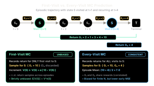
First-visit Monte Carlo averages returns only from the first time a state occurs in each episode to ensure strictly unbiased value estimates, whereas every-visit Monte Carlo averages returns from every appearance to harvest more data at the cost of transient bias.

First-visit Monte Carlo estimates state values using only the return after state S first appears in an episode, whereas every-visit Monte Carlo records returns after every occurrence.

Why Does This Exist?

In reinforcement learning, policy evaluation seeks to estimate the state-value function $V^\pi(s)$ —the expected cumulative discounted reward an agent receives when starting in state $s$ and following policy $\pi$ thereafter. Monte Carlo (MC) prediction solves this model-free by simulating complete trajectories through the environment, accumulating the observed rewards, and computing empirical sample averages.

However, in any realistic episodic environment featuring loops, cycles, or recurring conditions (such as grid navigation, robot locomotion, or financial trading sessions), an agent frequently revisits the same state $s$ multiple times within a single episode.

This recurring visit creates a fundamental algorithmic question: when state $s$ appears at time step $t_1$ and again at time step $t_2$ in the same trajectory, which downstream returns should update $V(s)$ ?

First-Visit MC considers only the return observed after the initial arrival at state $s$ during that episode, discarding subsequent visits.
Every-Visit MC treats every arrival at state $s$ as a valid sample point, averaging all corresponding returns across the trajectory.

Without this distinction, practitioners risk misinterpreting convergence guarantees, sample independence, and estimation variance. First-visit yields an independent, strictly unbiased estimator, while every-visit harvests more sample points per trajectory, trading finite-sample bias for reduced initial mean squared error (MSE).

Think of It Like This

Surveying Patient Hospital Stays

Imagine a regional healthcare director surveying patient satisfaction across various departments to evaluate quality of care. Some chronic patients check into the same specialized clinic multiple times during a single hospital stay (for example, triage upon arrival, a medication review at midday, and a final check-in before discharge).

In a First-Visit survey protocol, the clinic gives the patient an evaluation questionnaire only once: during their very first arrival. That single score reflects their entire subsequent hospital journey. Because each admitted patient contributes at most one survey response per admission, each entry comes from a separate, independent individual. The resulting average is a strictly unbiased metric of patient satisfaction, free from duplicate response skew.

In an Every-Visit survey protocol, the clinic hands the patient a feedback tablet at every single check-in counter throughout the day. If a patient visits the clinic three times, they submit three separate satisfaction ratings, all tied to the same overall stay. The hospital gathers three times as much data in the first week, but those three responses are not independent—an unusually pleasant or terrible discharge event correlates with and colors every response submitted during that stay.

Where the analogy stops: In a hospital survey, patient psychology, fatigue, or mood may evolve across check-ins. In reinforcement learning, the environment remains a Markov Decision Process (MDP): state transitions satisfy the Markov property, and the returns following each state visit are exact discounted sums of future rewards generated by the environment's transition dynamics and the stationary policy $\pi$ .

How It Actually Works

Mathematical Formulation and Return Estimation

Consider an episodic Markov Decision Process. Under policy $\pi$ , an episode generates a sequence of states, actions, and scalar rewards terminating at time step $T$ :

$S_0, A_0, R_1, S_1, A_1, R_2, \dots, S_{T-1}, A_{T-1}, R_T, S_T$

The discounted return $G_t$ following time step $t$ is the sum of future rewards discounted by factor $\gamma \in [0, 1]$ :

$G_t = \sum_{k=0}^{T - t - 1} \gamma^k R_{t + k + 1} = R_{t+1} + \gamma R_{t+2} + \gamma^2 R_{t+3} + \dots + \gamma^{T-t-1} R_T$

The true state-value function is defined as the conditional expectation:

$V^\pi(s) = \mathbb{E}_\pi \left[ G_t \;\middle|\; S_t = s \right]$

1. First-Visit Monte Carlo Prediction

In first-visit MC, we record the return $G_t$ if and only if time step $t$ is the first time state $s$ appears in that specific episode. Let $\mathcal{T}_1^{(e)}(s)$ denote the earliest time step state $s$ was visited in episode $e$ :

$\mathcal{T}_1^{(e)}(s) = \min \{ t \in \{0, 1, \dots, T^{(e)}-1\} : S_t^{(e)} = s \}$

If state $s$ never appears in episode $e$ , the set is empty. Over a collection of $M$ episodes, the first-visit estimate $V_{\text{FV}}(s)$ is the average of returns following these first visits:

$V_{\text{FV}}(s) = \frac{\sum_{e=1}^M \mathbb{I}(s \in \tau^{(e)}) G_{\mathcal{T}_1^{(e)}(s)}^{(e)}}{\sum_{e=1}^M \mathbb{I}(s \in \tau^{(e)})}$

where $\mathbb{I}(s \in \tau^{(e)})$ is an indicator function equal to $1$ if episode $e$ visited state $s$ , and $0$ otherwise.

Statistical Property: Because each episode contributes at most one return to $V(s)$ , and trajectories generated across independent episodes are mutually independent, the sampled returns $\{G_{\mathcal{T}_1^{(e)}(s)}^{(e)}\}$ are independent and identically distributed (i.i.d.) random variables.
Unbiasedness: $\mathbb{E}[V_{\text{FV}}(s)] = V^\pi(s)$ for any number of sampled episodes.
Asymptotic Convergence: By the Strong Law of Large Numbers, $V_{\text{FV}}(s) \xrightarrow{a.s.} V^\pi(s)$ as $M \to \infty$ . The variance of the estimate scales as $\mathcal{O}(1 / M)$ .

2. Every-Visit Monte Carlo Prediction

In every-visit MC, we record the return $G_t$ for every time step $t$ where state $s$ occurs, regardless of whether it has been visited earlier in that same episode:

$\mathcal{T}_{\text{all}}^{(e)}(s) = \{ t \in \{0, 1, \dots, T^{(e)}-1\} : S_t^{(e)} = s \}$

The every-visit estimate $V_{\text{EV}}(s)$ averages all sampled returns across all visits:

$V_{\text{EV}}(s) = \frac{\sum_{e=1}^M \sum_{t \in \mathcal{T}_{\text{all}}^{(e)}(s)} G_t^{(e)}}{\sum_{e=1}^M |\mathcal{T}_{\text{all}}^{(e)}(s)|}$

Statistical Property: When state $s$ occurs multiple times in episode $e$ at times $t_a < t_b$ , the returns $G_{t_a}$ and $G_{t_b}$ share downstream rewards: $G_{t_a} = \sum_{k=0}^{t_b - t_a - 1} \gamma^k R_{t_a + k + 1} + \gamma^{t_b - t_a} G_{t_b}$ Because $G_{t_a}$ directly contains $G_{t_b}$ , the returns are statistically correlated.
Transient Bias: Due to intra-episode correlation, $V_{\text{EV}}(s)$ is a biased estimator for finite sample sizes ( $\mathbb{E}[V_{\text{EV}}(s)] \neq V^\pi(s)$ ).
Consistency: Despite finite-sample bias, every-visit MC is asymptotically consistent ( $V_{\text{EV}}(s) \xrightarrow{a.s.} V^\pi(s)$ as $M \to \infty$ ). Because it extracts more return samples per trajectory, its Mean Squared Error (MSE) is often lower than first-visit MC during early iterations.

3. Incremental Implementation

Both algorithms can be implemented incrementally without storing complete lists of returns in memory. At each recorded visit to state $s$ with return $G_t$ :

$N(s) \leftarrow N(s) + 1$

$V(s) \leftarrow V(s) + \frac{1}{N(s)} \left[ G_t - V(s) \right]$

For non-stationary tasks where policy $\pi$ or environment dynamics drift, the sample-average step size $1 / N(s)$ is replaced by a fixed learning rate $\alpha \in (0, 1]$ :

$V(s) \leftarrow V(s) + \alpha \left[ G_t - V(s) \right]$

Worked numerical example

Consider an environment with states $\{S_1, S_2, \text{Terminal}\}$ and undiscounted returns ( $\gamma = 1.0$ ). Value functions and visit counters are initialized to zero: $V(S_1) = 0, V(S_2) = 0$ , and $N(S_1) = 0, N(S_2) = 0$ .

Episode 1

An agent executes policy $\pi$ and generates the following trajectory:

$t=0$ : Starts in $S_1$ , takes an action, receives reward $R_1 = +2$ , transitions to $S_2$ .
$t=1$ : In $S_2$ , takes an action, receives reward $R_2 = +3$ , transitions back to $S_1$ .
$t=2$ : In $S_1$ (second visit!), takes an action, receives reward $R_3 = +5$ , transitions to Terminal state $T$ .

Computing returns working backward from termination:

At $t=2$ ( $S_1$ , second visit): $G_2 = R_3 = 5.0$
At $t=1$ ( $S_2$ , first visit): $G_1 = R_2 + G_2 = 3.0 + 5.0 = 8.0$
At $t=0$ ( $S_1$ , first visit): $G_0 = R_1 + G_1 = 2.0 + 8.0 = 10.0$

First-Visit Updates for Episode 1:

State $S_1$ : First visit occurs at $t=0$ with $G_0 = 10.0$ . The second visit at $t=2$ is ignored. $N_{\text{FV}}(S_1) \leftarrow 0 + 1 = 1$ $V_{\text{FV}}(S_1) \leftarrow 0.0 + \frac{1}{1}(10.0 - 0.0) = 10.0$
State $S_2$ : First visit occurs at $t=1$ with $G_1 = 8.0$ . $N_{\text{FV}}(S_2) \leftarrow 0 + 1 = 1$ $V_{\text{FV}}(S_2) \leftarrow 0.0 + \frac{1}{1}(8.0 - 0.0) = 8.0$

Every-Visit Updates for Episode 1:

State $S_1$ $S_{1}$ : Updates on both occurrences ( $t=0$ $t = 0$ and $t=2$ $t = 2$ ).
- First occurrence ( $t=0$ ): $N_{\text{EV}}(S_1) \leftarrow 1, \quad V_{\text{EV}}(S_1) \leftarrow 0.0 + \frac{1}{1}(10.0 - 0.0) = 10.0$
- Second occurrence ( $t=2$ ): $N_{\text{EV}}(S_1) \leftarrow 2, \quad V_{\text{EV}}(S_1) \leftarrow 10.0 + \frac{1}{2}(5.0 - 10.0) = 7.5$
- Equivalent batch average: $\frac{10.0 + 5.0}{2} = 7.5$
State $S_2$ : Updates on the single visit at $t=1$ . $N_{\text{EV}}(S_2) \leftarrow 1, \quad V_{\text{EV}}(S_2) \leftarrow 8.0$

Episode 2

The agent collects a second trajectory:

$t=0$ : Starts in $S_2$ , receives reward $R_1 = +4$ , transitions to $S_1$ .
$t=1$ : In $S_1$ , receives reward $R_2 = +2$ , transitions to Terminal state $T$ .

Computing returns working backward:

At $t=1$ ( $S_1$ ): $G_1 = R_2 = 2.0$
At $t=0$ ( $S_2$ ): $G_0 = R_1 + G_1 = 4.0 + 2.0 = 6.0$

First-Visit Updates after Episode 2:

State $S_1$ : First visit in Episode 2 is at $t=1$ with $G_1 = 2.0$ . $N_{\text{FV}}(S_1) \leftarrow 1 + 1 = 2$ $V_{\text{FV}}(S_1) \leftarrow 10.0 + \frac{1}{2}(2.0 - 10.0) = 6.0$
State $S_2$ : First visit in Episode 2 is at $t=0$ with $G_0 = 6.0$ . $N_{\text{FV}}(S_2) \leftarrow 1 + 1 = 2$ $V_{\text{FV}}(S_2) \leftarrow 8.0 + \frac{1}{2}(6.0 - 8.0) = 7.0$

Every-Visit Updates after Episode 2:

State $S_1$ $S_{1}$ : One visit occurs at $t=1$ $t = 1$ with $G_1 = 2.0$ $G_{1} = 2.0$ . $N_{\text{EV}}(S_1) \leftarrow 2 + 1 = 3$ $N_{EV} (S_{1}) \leftarrow 2 + 1 = 3$ $V_{\text{EV}}(S_1) \leftarrow 7.5 + \frac{1}{3}(2.0 - 7.5) = 7.5 - 1.833 = 5.67$ $V_{EV} (S_{1}) \leftarrow 7.5 + \frac{1}{3} (2.0 - 7.5) = 7.5 - 1.833 = 5.67$
- Batch verification: $\frac{10.0 + 5.0 + 2.0}{3} = \frac{17.0}{3} \approx 5.67$
State $S_2$ : One visit occurs at $t=0$ with $G_0 = 6.0$ . $N_{\text{EV}}(S_2) \leftarrow 1 + 1 = 2$ $V_{\text{EV}}(S_2) \leftarrow 8.0 + \frac{1}{2}(6.0 - 8.0) = 7.0$

Notice how $V(S_2)$ evaluates to identically $7.0$ in both methods because $S_2$ was never revisited within either episode. In contrast, $V(S_1)$ diverges ( $6.00$ vs $5.67$ ) because Every-Visit incorporated the intermediate sub-trajectory return $G_2 = 5.0$ .

Code

1from typing import Dict, List, Tuple2
3
4def first_visit_mc_prediction(5    episodes: List[List[Tuple[str, float]]],6    gamma: float = 1.0,7) -> Dict[str, float]:8    """Estimate state values using First-Visit Monte Carlo prediction.9
10    Args:11        episodes: List of trajectories, where each trajectory is a list of12            (state, reward) tuples representing (S_t, R_{t+1}) up to termination.13        gamma: Discount factor in [0, 1].14
15    Returns:16        Dictionary mapping each visited state to its estimated value V(s).17    """18    returns_sum: Dict[str, float] = {}19    returns_count: Dict[str, int] = {}20
21    for episode in episodes:22        # Step 1: Work backward to calculate return G_t for each step23        G = 0.024        T = len(episode)25        step_returns: List[Tuple[str, float]] = []26
27        for t in reversed(range(T)):28            state, reward = episode[t]29            G = gamma * G + reward30            step_returns.append((state, G))31
32        # Reverse back to forward chronological order (t = 0 ... T-1)33        step_returns.reverse()34
35        # Step 2: Track states visited in this episode; update on first occurrence only36        visited_in_episode = set()37        for state, G_t in step_returns:38            if state not in visited_in_episode:39                visited_in_episode.add(state)40                returns_sum[state] = returns_sum.get(state, 0.0) + G_t41                returns_count[state] = returns_count.get(state, 0) + 142
43    return {s: returns_sum[s] / returns_count[s] for s in returns_sum}44
45
46def every_visit_mc_prediction(47    episodes: List[List[Tuple[str, float]]],48    gamma: float = 1.0,49) -> Dict[str, float]:50    """Estimate state values using Every-Visit Monte Carlo prediction.51
52    Args:53        episodes: List of trajectories, where each trajectory is a list of54            (state, reward) tuples representing (S_t, R_{t+1}) up to termination.55        gamma: Discount factor in [0, 1].56
57    Returns:58        Dictionary mapping each visited state to its estimated value V(s).59    """60    returns_sum: Dict[str, float] = {}61    returns_count: Dict[str, int] = {}62
63    for episode in episodes:64        # Step 1: Work backward to calculate return G_t for each step65        G = 0.066        T = len(episode)67
68        # In every-visit, every step update can accumulate directly69        for t in reversed(range(T)):70            state, reward = episode[t]71            G = gamma * G + reward72            returns_sum[state] = returns_sum.get(state, 0.0) + G73            returns_count[state] = returns_count.get(state, 0) + 174
75    return {s: returns_sum[s] / returns_count[s] for s in returns_sum}76
77
78if __name__ == "__main__":79    # Trajectories matching the worked numerical example:80    # Episode 1: S1 -(r=2)-> S2 -(r=3)-> S1 -(r=5)-> Terminal81    # Episode 2: S2 -(r=4)-> S1 -(r=2)-> Terminal82    sample_episodes: List[List[Tuple[str, float]]] = [83        [("S1", 2.0), ("S2", 3.0), ("S1", 5.0)],84        [("S2", 4.0), ("S1", 2.0)],85    ]86
87    v_first = first_visit_mc_prediction(sample_episodes, gamma=1.0)88    v_every = every_visit_mc_prediction(sample_episodes, gamma=1.0)89
90    print("--- First-Visit MC Value Estimates ---")91    for state in sorted(v_first):92        print(f"V_FV({state}) = {v_first[state]:.2f}")93
94    print("\n--- Every-Visit MC Value Estimates ---")95    for state in sorted(v_every):96        print(f"V_EV({state}) = {v_every[state]:.2f}")

1--- First-Visit MC Value Estimates ---2V_FV(S1) = 6.003V_FV(S2) = 7.004
5--- Every-Visit MC Value Estimates ---6V_EV(S1) = 5.677V_EV(S2) = 7.00

Watch Out For

High variance of Monte Carlo returns requiring hundreds of complete episodes before values stabilize

Because Monte Carlo estimation computes return $G_t$ as the raw sum of all rewards from step $t$ until the terminal state without any intermediate bootstrapping, every random transition and stochastic reward along the rest of the trajectory compounds into $G_t$ .

In tasks with long horizons ( $T > 100$ ) or noisy rewards, returns exhibit extreme sample variance. If an agent attempts to perform control (policy iteration) using value estimates built from only a few dozen episodes, noisy return fluctuations will corrupt the greedy policy improvements, locking the policy into suboptimal behaviors.

Symptom: Value functions swing wildly between evaluation batches, and policy improvement steps fail to stabilize or repeatedly oscillate.

Concrete Fix: Either collect hundreds to thousands of episodes before updating policies, incorporate discount factors $\gamma < 1.0$ to damp distant reward noise, or switch to bootstrapping Temporal Difference methods such as TD(0) or n-step TD which replace distal stochasticity with value estimates $V(S_{t+1})$ .

Correlated intra-episode returns introducing transient bias in small datasets

Every-visit Monte Carlo incorporates multiple returns from the same episode when states recur. If a small dataset contains an outlier episode where an agent gets trapped in a cycle before receiving a large penalty or reward, every-visit MC counts that single anomalous trajectory multiple times for each recurring state.

Symptom: In small-sample regimes ( $M < 30$ ), recurring states display severe overestimation or underestimation bias, deviating significantly from the true expected value $V^\pi(s)$ .

Concrete Fix: When evaluating policies on small historical logs where strict unbiasedness is required, use First-Visit MC. Reserve Every-Visit MC for high-throughput environments where sample volume is large enough for asymptotic consistency to dominate.

The Quick Version

First-Visit MC averages the return following only the initial visit to state $s$ per episode, yielding a strictly unbiased estimator ( $\mathbb{E}[V(s)] = V^\pi(s)$ ) with i.i.d. return samples.
Every-Visit MC averages returns from all occurrences of state $s$ in an episode; although intra-episode correlation introduces finite-sample bias, it is asymptotically consistent and often lowers early mean squared error.
Both algorithms converge to the true value function $V^\pi(s)$ as the number of sampled episodes approaches infinity by the Law of Large Numbers.
Because both methods rely on complete episodic returns without bootstrapping, they require terminating environments and experience higher sample variance than Temporal Difference learning.