Monte Carlo Action Values

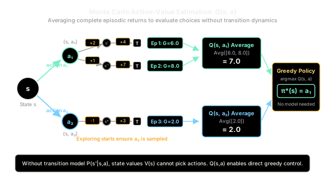
Estimating state values alone cannot guide decisions when transition dynamics are unknown. Monte Carlo action-value estimation records the total returns following specific choices in each state, learning the expected payout of every action purely from experience.

Monte Carlo action-value estimation samples complete episodic rollouts from state-action pairs to compute empirical averages Q(s, a) without transition dynamics.

Why Does This Exist?

In reinforcement learning, the ultimate objective is finding an optimal policy that maximizes cumulative reward. When an agent possesses a complete environment model—namely the transition probabilities $P(s' \mid s, a)$ and expected rewards $R(s, a, s')$ —state values $V(s)$ are entirely sufficient to select the best action via a standard one-step lookahead:

$\pi^*(s) = \arg\max_{a \in \mathcal{A}} \sum_{s'} P(s' \mid s, a) \left[ R(s, a, s') + \gamma V(s') \right]$

However, in model-free reinforcement learning, the environment is an unknown black box. Even if an oracle provides the true state values $V(s')$ , the agent cannot act greedily because it has no mathematical model specifying which action $a$ leads to which successor state $s'$ . Knowing that state $s'$ is worth $+100$ is useless if you do not know which joystick movement lands you there.

Action values $Q(s, a)$ resolve this fundamental dilemma. By estimating the expected return of taking a specific action $a$ in state $s$ and thereafter following policy $\pi$ , the agent can select actions greedily with a direct maximum:

$\pi'(s) = \arg\max_{a \in \mathcal{A}} Q(s, a)$

Monte Carlo estimation evaluates these action values directly from episodic experience. It eliminates the need for transition models or bootstrapping, but it introduces an essential structural requirement: while an agent naturally visits states along a trajectory, estimating all actions requires active exploration so every alternative action from each state is repeatedly sampled.

Think of It Like This

The Restaurant Tasting Menu Pairing

Imagine you are dining through a multi-course chef's tasting menu at a fine restaurant, but the kitchen refuses to give you the recipes or explain the culinary science behind each dish.

When Course 3 arrives (State $s$ : pan-seared sea bass), the server offers you a choice between two beverage pairings: Pinot Noir (Action $a_1$ ) or Chardonnay (Action $a_2$ ).

Knowing that Course 3 is generally rated $8.5/10$ by critics (State Value $V(s)$ ) does not help you choose your drink. Because you do not know the chemical interactions between the wine and the sauce (the environment transition model $P$ ), you cannot mentally predict the final outcome before tasting it.

To estimate the action values, you must experience the meal directly:

On night one, you order Chardonnay ( $a_2$ ). You drink the wine, finish the remaining courses through dessert (the terminal state), and rate your full evening satisfaction score ( $G^{(1)} = +6.2$ ).
On night two, you order Pinot Noir ( $a_1$ ) with the same fish course, complete the dinner, and record your evening satisfaction score ( $G^{(2)} = +5.6$ ).
Over repeated visits, you average the total satisfaction scores resulting from each specific beverage decision. The resulting averages are your empirical action values: $Q(\text{Sea Bass}, \text{Chardonnay})$ and $Q(\text{Sea Bass}, \text{Pinot Noir})$ .

Once you have these averages, choosing your drink next time is effortless: simply select the beverage with the higher empirical score—no sommelier needed.

Where the analogy stops: Human diners evaluate meals using holistic taste memories and sensory fatigue, whereas reinforcement learning computes a mathematically discounted return $\sum \gamma^t R_{t+1}$ . Furthermore, a diner can generalize from prior culinary knowledge, whereas tabular Monte Carlo methods require resetting and rerunning dozens of complete episodes from scratch across every state-action combination to eliminate sample variance.

How It Actually Works

Action-Value Formulation and Return Sampling

Given a Markov Decision Process defined by state space $\mathcal{S}$ , action space $\mathcal{A}$ , discount factor $\gamma \in [0, 1]$ , and terminal time step $T$ , the action-value function under policy $\pi$ is the expected total discounted return starting from state $s$ , taking action $a$ :

$Q^\pi(s, a) \doteq \mathbb{E}_\pi \left[ G_t \;\middle|\; S_t = s, A_t = a \right] = \mathbb{E}_\pi \left[ \sum_{k=0}^{T - t - 1} \gamma^k R_{t+k+1} \;\middle|\; S_t = s, A_t = a \right]$

Here:

$S_t \in \mathcal{S}$ represents the state at time step $t$ .
$A_t \in \mathcal{A}$ represents the action executed at time step $t$ .
$R_{t+k+1} \in \mathbb{R}$ is the numerical reward obtained at step $t+k+1$ .
$\gamma \in [0, 1]$ is the discount factor balancing short-term and long-term gains.
$G_t$ is the actual accumulated discounted return from time step $t$ through terminal step $T$ .

In First-Visit Monte Carlo estimation of action values, the agent executes complete episodes following policy $\pi$ . For each episode trajectory:

$\tau = (S_0, A_0, R_1, S_1, A_1, R_2, \dots, S_{T-1}, A_{T-1}, R_T, S_T)$

the agent moves from $t = T-1$ backward to $t = 0$ , accumulating returns $G_t = R_{t+1} + \gamma G_{t+1}$ . For every state-action pair $(s, a)$ , the return $G_t$ is recorded only if time step $t$ is the first occurrence of $(s, a)$ in that episode.

The tabular value estimate $Q(s, a)$ is updated as the arithmetic mean of all recorded returns:

$Q(s, a) = \frac{1}{|\text{Returns}(s, a)|} \sum_{G \in \text{Returns}(s, a)} G$

Equivalently, the update can be performed incrementally using a visit counter $N(s, a)$ :

$N(s, a) \leftarrow N(s, a) + 1$

$Q(s, a) \leftarrow Q(s, a) + \frac{1}{N(s, a)} \left( G_t - Q(s, a) \right)$

Because a deterministic policy $\pi$ would repeatedly select the exact same action from state $s$ , many state-action pairs would never be experienced ( $N(s, a) = 0$ ). To guarantee convergence across all choices, Monte Carlo prediction relies on Exploring Starts: every episode begins with a state-action pair $(S_0, A_0)$ sampled such that every combination has a non-zero probability:

$P(S_0 = s, A_0 = a) > 0 \quad \forall s \in \mathcal{S}, \; a \in \mathcal{A}$

Worked numerical example

Consider an agent learning action values for starting state $s_0$ with two available actions $\mathcal{A} = \{a_1, a_2\}$ under discount factor $\gamma = 0.90$ . Initially, tables are empty: $Q(s_0, a) = 0.0$ and $N(s_0, a) = 0$ for all $a$ .

Three successive episodes are generated:

Episode 1 (Exploring start: $s_0, a_1$ )

Trajectory: $(s_0, a_1, R_1 = +2.0) \to (s_1, a_1, R_2 = +4.0) \to \text{Terminal}$
Return from step 0: $G_0 = R_1 + \gamma R_2 = 2.0 + 0.90 \times 4.0 = 2.0 + 3.60 = 5.60$
First visit to $(s_0, a_1)$ : $N(s_0, a_1) = 1$ $Q(s_0, a_1) = 0.0 + \frac{1}{1}(5.60 - 0.0) = 5.600$

Episode 2 (Exploring start: $s_0, a_2$ )

Trajectory: $(s_0, a_2, R_1 = -1.0) \to (s_2, a_2, R_2 = +8.0) \to \text{Terminal}$
Return from step 0: $G_0 = R_1 + \gamma R_2 = -1.0 + 0.90 \times 8.0 = -1.0 + 7.20 = 6.20$
First visit to $(s_0, a_2)$ : $N(s_0, a_2) = 1$ $Q(s_0, a_2) = 0.0 + \frac{1}{1}(6.20 - 0.0) = 6.200$

Episode 3 (Start: $s_0, a_1$ )

Trajectory: $(s_0, a_1, R_1 = +3.0) \to (s_1, a_2, R_2 = +1.0) \to \text{Terminal}$
Return from step 0: $G_0 = R_1 + \gamma R_2 = 3.0 + 0.90 \times 1.0 = 3.0 + 0.90 = 3.90$
First visit to $(s_0, a_1)$ in this episode: $N(s_0, a_1) = 2$ $Q(s_0, a_1) \leftarrow 5.600 + \frac{1}{2}(3.90 - 5.600) = 5.600 - 0.850 = 4.750$

Resulting Policy Decision

At state $s_0$ , the agent compares the empirical estimates:

$Q(s_0, a_1) = \frac{5.60 + 3.90}{2} = 4.750$
$Q(s_0, a_2) = \frac{6.20}{1} = 6.200$

Selecting greedily without needing transition dynamics:

$\pi^*(s_0) = \arg\max_{a \in \{a_1, a_2\}} Q(s_0, a) = a_2$

Because Episode 2 enforced an exploring start on $a_2$ , the agent discovered that $a_2$ yielded an expected payout of $6.200$ , outperforming $a_1$ ( $4.750$ ).

Code

1from typing import Dict, List, NamedTuple, Tuple2
3class Transition(NamedTuple):4    state: str5    action: str6    reward: float7
8Episode = List[Transition]9
10def first_visit_mc_action_values(11    episodes: List[Episode],12    gamma: float = 0.9013) -> Tuple[Dict[Tuple[str, str], float], Dict[Tuple[str, str], int]]:14    """15    Computes Q(s, a) tabular action values using First-Visit Monte Carlo prediction.16
17    Args:18        episodes: List of completed episodes containing state-action-reward transitions.19        gamma: Discount factor in range [0, 1].20
21    Returns:22        q_table: Dictionary mapping (state, action) pairs to their estimated Q-value.23        counts: Dictionary mapping (state, action) pairs to total first-visit counts.24    """25    q_table: Dict[Tuple[str, str], float] = {}26    returns_sum: Dict[Tuple[str, str], float] = {}27    counts: Dict[Tuple[str, str], int] = {}28
29    for episode in episodes:30        g: float = 0.031        # Step backward from the terminal transition to accumulate discounted returns32        backward_returns: List[Tuple[str, str, float]] = []33        for step in reversed(episode):34            g = step.reward + gamma * g35            backward_returns.append((step.state, step.action, g))36        37        # Restore chronological order38        backward_returns.reverse()39
40        # Track first visits within this specific episode41        visited_in_episode = set()42        for state, action, return_val in backward_returns:43            sa_pair = (state, action)44            if sa_pair not in visited_in_episode:45                visited_in_episode.add(sa_pair)46                47                if sa_pair not in counts:48                    counts[sa_pair] = 049                    returns_sum[sa_pair] = 0.050
51                counts[sa_pair] += 152                returns_sum[sa_pair] += return_val53                # Empirical mean of all observed returns54                q_table[sa_pair] = returns_sum[sa_pair] / counts[sa_pair]55
56    return q_table, counts57
58# Simulated episodes matching the worked example59episodes_dataset: List[Episode] = [60    # Episode 1: (s0, a1) -> (s1, a1) -> Terminal61    [Transition("s0", "a1", 2.0), Transition("s1", "a1", 4.0)],62    # Episode 2: (s0, a2) -> (s2, a2) -> Terminal (Exploring start)63    [Transition("s0", "a2", -1.0), Transition("s2", "a2", 8.0)],64    # Episode 3: (s0, a1) -> (s1, a2) -> Terminal65    [Transition("s0", "a1", 3.0), Transition("s1", "a2", 1.0)],66]67
68q_values, visit_counts = first_visit_mc_action_values(episodes_dataset, gamma=0.90)69
70# Evaluate learned action values at state s071print("--- Learned Monte Carlo Action Values at s0 ---")72for action in ["a1", "a2"]:73    pair = ("s0", action)74    val = q_values.get(pair, 0.0)75    cnt = visit_counts.get(pair, 0)76    print(f"Q(s0, {action}) = {val:.3f} | Visits: {cnt}")77
78greedy_action = max(["a1", "a2"], key=lambda a: q_values.get(("s0", a), float("-inf")))79print(f"Greedy Policy Selection: pi*(s0) = {greedy_action}")80
81# Expected Output:82# --- Learned Monte Carlo Action Values at s0 ---83# Q(s0, a1) = 4.750 | Visits: 284# Q(s0, a2) = 6.200 | Visits: 185# Greedy Policy Selection: pi*(s0) = a2

Watch Out For

Action Starvation: The Greedy Policy Trap

When estimating action values to guide decisions, following a greedy policy creates a destructive feedback loop: actions with higher initial estimates are repeatedly executed, while alternative actions receive zero subsequent visits ( $N(s, a) = 0$ ).

Symptom: The Q-estimates for untried or lower-rated actions freeze permanently. If a stochastic transition gave an optimal action an unlucky negative reward on its very first trial, the agent will never select it again, locking into a suboptimal policy for the lifetime of the system.

The Fix: You cannot evaluate action values under a purely deterministic greedy policy without active exploration mechanisms:

In episodic simulation, initialize episodes with Exploring Starts, guaranteeing uniform non-zero probability for every state-action pair $(S_0, A_0)$ .
In online environments where starting pairs cannot be set arbitrarily, use stochastic exploratory policies such as $\varepsilon$ -greedy exploration (choosing a random uniform action with probability $\varepsilon$ ) or softmax exploration. This guarantees infinite visits to every $(s, a)$ pair as episode counts approach infinity.

The Quick Version

Model-free control prerequisite: Unlike state values $V(s)$ , action values $Q(s, a)$ do not require transition dynamics $P(s' \mid s, a)$ to select greedy actions.
Empirical return averaging: Monte Carlo computes $Q(s, a)$ by taking the average of observed total returns following the execution of action $a$ in state $s$ across completed episodes.
First-visit rule: Updates use only the return from the initial encounter of $(s, a)$ within each episode, preventing cyclical bias while providing unbiased estimates.
Mandatory exploration: Because greedy policies starve unchosen actions of updates, reliable estimation requires exploring starts or $\varepsilon$ -greedy exploration to guarantee full state-action coverage.